Multivariate kernel density estimation

Kernel density estimation is a nonparametric technique for density estimation i.e., estimation of probability density functions, which is one of the fundamental questions in statistics. It can be viewed as a generalisation of histogram density estimation with improved statistical properties. Apart from histograms, other types of density estimators include parametric, spline, wavelet and Fourier series. Kernel density estimators were first introduced in the scientific literature for univariate data in the 1950s and 1960s^[1][2] and subsequently have been widely adopted. It was soon recognised that analogous estimators for multivariate data would be an important addition to multivariate statistics. Based on research carried out in the 1990s and 2000s, multivariate kernel density estimation has reached a level of maturity comparable to their univariate counterparts.^[3]

Motivation

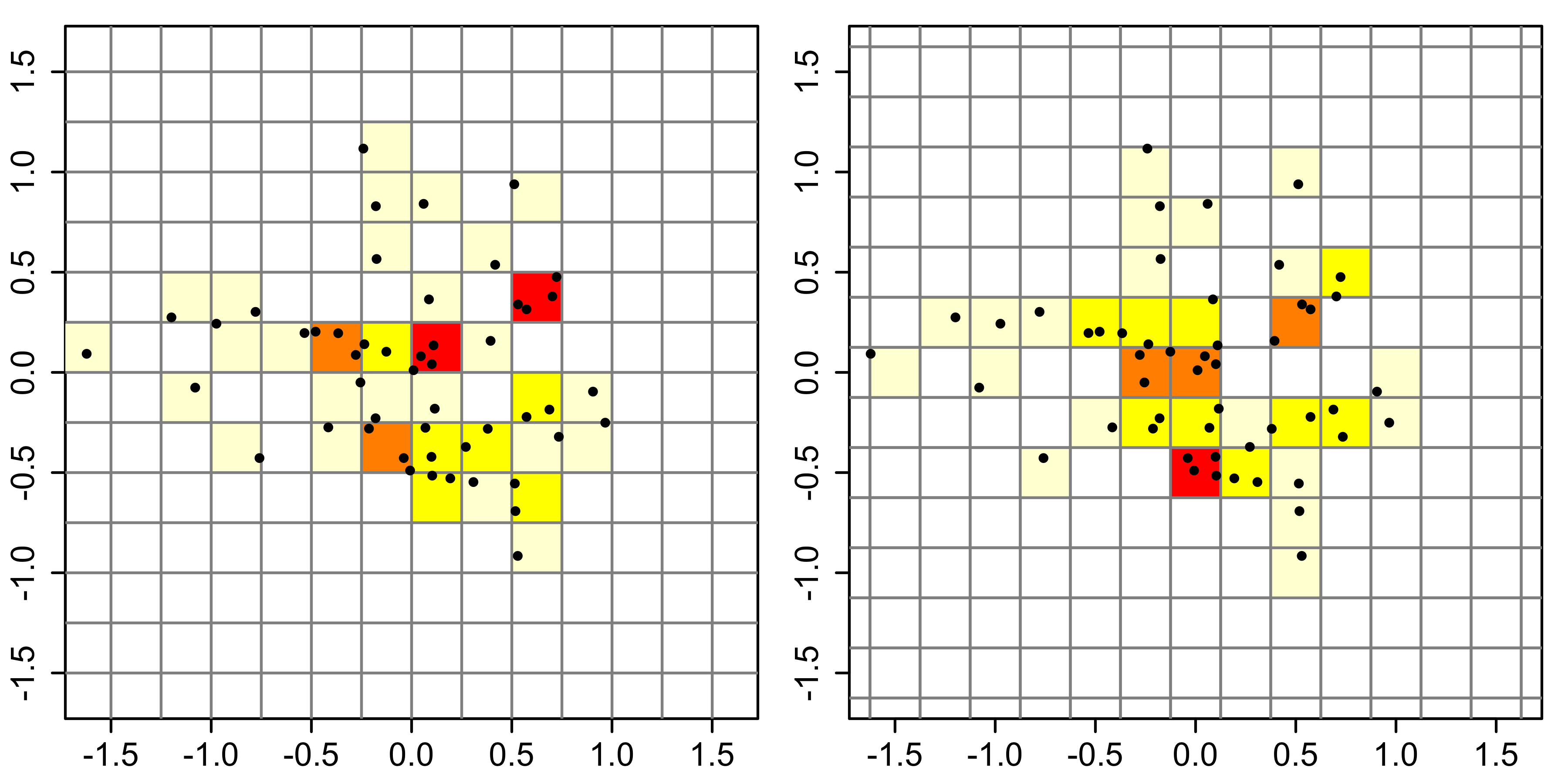
We take an illustrative synthetic bivariate data set of 50 points to illustrate the construction of histograms. This requires the choice of an anchor point (the lower left corner of the histogram grid). For the histogram on the left, we choose (−1.5, −1.5): for the one on the right, we shift the anchor point by 0.125 in both directions to (−1.625, −1.625). Both histograms have a binwidth of 0.5, so any differences are due to the change in the anchor point only. The colour coding indicates the number of data points which fall into a bin: 0=white, 1=pale yellow, 2=bright yellow, 3=orange, 4=red. The left histogram appears to indicate that the upper half has a higher density than the lower half, whereas it is the reverse is the case for the right-hand histogram, confirming that histograms are highly sensitive to the placement of the anchor point.^[4]

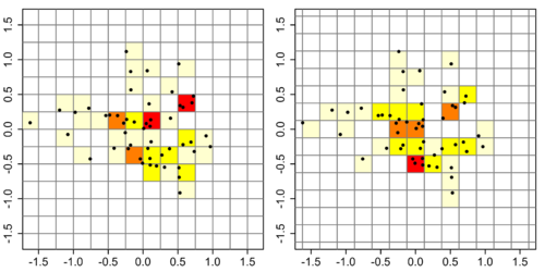Comparison of 2D histograms. Left. Histogram with anchor point at (−1.5, -1.5). Right. Histogram with anchor point at (−1.625, −1.625). Both histograms have a bin width of 0.5, so differences in appearances of the two histograms are due to the placement of the anchor point.

One possible solution to this anchor point placement problem is to remove the histogram binning grid completely. In the left figure below, a kernel (represented by the grey lines) is centred at each of the 50 data points above. The result of summing these kernels is given on the right figure, which is a kernel density estimate. The most striking difference between kernel density estimates and histograms is that the former are easier to interpret since they do not contain artifices induced by a binning grid. The coloured contours correspond to the smallest region which contains the respective probability mass: red = 25%, orange + red = 50%, yellow + orange + red = 75%, thus indicating that a single central region contains the highest density.

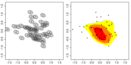Construction of 2D kernel density estimate. Left. Individual kernels. Right. Kernel density estimate.

The goal of density estimation is to take a finite sample of data and to make inferences about the underyling probability density function everywhere, including where no data are observed. In kernel density estimation, the contribution of each data point is smoothed out from a single point into a region of space surrounding it. Aggregating the individually smoothed contributions gives an overall picture of the structure of the data and its density function. In the details to follow, we show that this approach leads to a reasonable estimate of the underlying density function.

Definition

The previous figure is a graphical representation of kernel density estimate, which we now define in an exact manner. Let x₁, x₂, …, x_n be a sample of d-variate random vectors drawn from a common distribution described by the density function ƒ. The kernel density estimate is defined to be

$\hat{f}_\bold{H}(\bold{x})= \frac1n \sum_{i=1}^n K_\bold{H} (\bold{x} - \bold{x}_i)$

where

• x = (x₁, x₂, …, x_d)^T, x_i = (x_i1, x_i2, …, x_id)^T, i = 1, 2, …, n are d-vectors;
• H is the bandwidth (or smoothing) d×d matrix which is symmetric and positive definite;
• K is the kernel function which is a symmetric multivariate density;
• K_H(x) = |H|^−1/2 K(H^−1/2x).

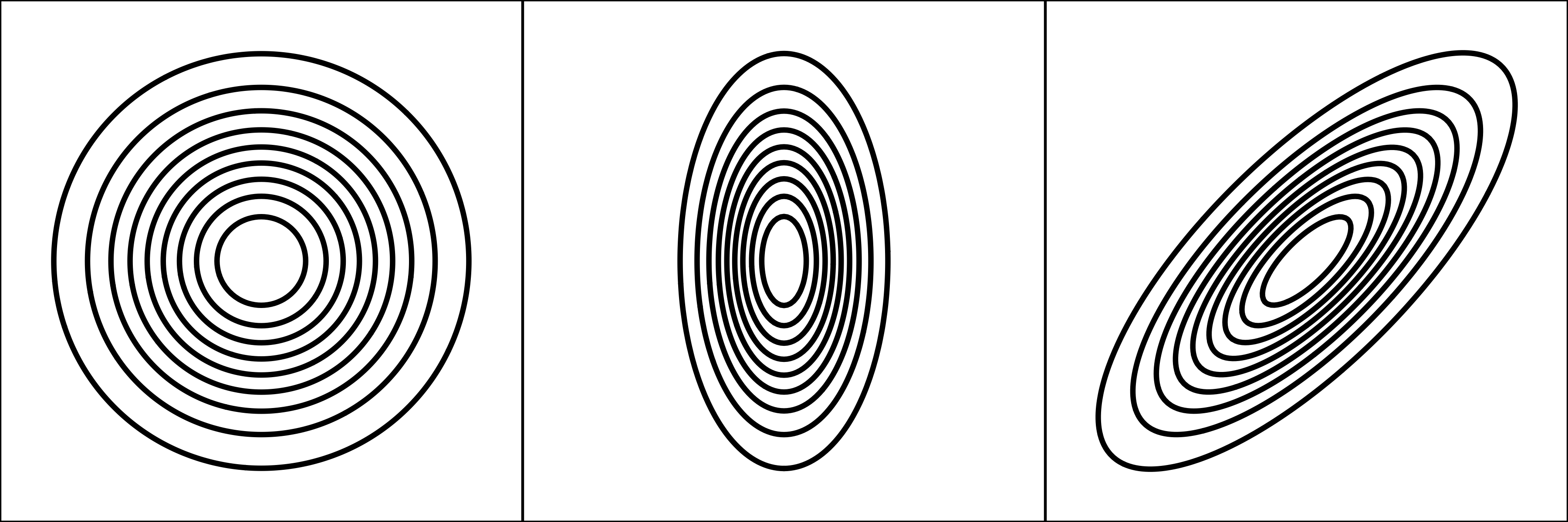
The choice of the kernel function K is not crucial to the accuracy of kernel density estimators, so we use the standard multivariate normal kernel throughout: K(x) = (2π)^−d/2 exp(−¹⁄₂x^Tx). Whereas the choice of the bandwidth matrix H is the single most important factor affecting its accuracy since it controls the amount of and orientation of smoothing induced.^[5]:36–39 That the bandwidth matrix also induces an orientation is a basic difference between multivariate kernel density estimation from its univariate analogue since orientation is not defined for 1D kernels. This leads to the choice of the parametrisation of this bandwidth matrix. The three main parametrisation classes (in increasing order of complexity) are S, the class of positive scalars times the identity matrix; D, diagonal matrices with positive entries on the main diagonal; and F, symmetric positive definite matrices. The S class kernels have the same amount of smoothing applied in all coordinate directions, D kernels allow different amounts of smoothing in each of the coordinates, and F kernels allow arbitrary amounts and orientation of the smoothing. Historically S and D kernels are the most widespread due to computational reasons, but research indicates that important gains in accuracy can be obtained using the more general F class kernels^[6][7].

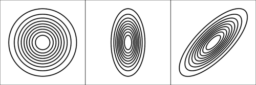Comparison of the three main bandwidth matrix parametrisation classes. Left. S positive scalar times the identity matrix. Centre. D diagonal matrix with positive entries on the main diagonal. Right. F symmetric positive definite matrix.

Optimal bandwidth matrix selection

The most commonly used optimality criterion for selecting a bandwidth matrix is the MISE or mean integrated squared error

$\operatorname{MISE} (\bold{H}) = \operatorname{E}\!\left[\, \int (\hat{f}_\bold{H} (\bold{x}) - f(\bold{x}))^2 \, d\bold{x} \;\right].$

This in general does not possess a closed-form expression, so it is usual to use its asymptotic approximation (AMISE) as a proxy

$\operatorname{AMISE} (\bold{H}) = n^{-1} |\bold{H}|^{-1/2} R(K) + \tfrac{1}{4} m_2(K)^2 (\operatorname{vec}^T \bold{H}) \bold{\Psi}_4 (\operatorname{vec}^T \bold{H})$

where

• $R(K) = \int K(\bold{x})^2 \, d\bold{x}$, with R(K) = (4π)^−d/2 when K is a normal kernel
• $\int \bold{x} \bold{x}^T K(\bold{x})^2 \, d\bold{x} = m_2(K) \bold{I}_d$, with I_d being the d × d identity matrix, with m₂ = 1 for the normal kernel
• D²ƒ is the d × d Hessian matrix of second order partial derivatives of ƒ
• $\bold{\Psi}_4 = \int (\operatorname{vec} \, \operatorname{D}^2 f(\bold{x})) (\operatorname{vec}^T \operatorname{D}^2 f(\bold{x})) \, d\bold{x}$ is a d² × d² matrix of integrated fourth order partial derivatives of ƒ
• vec is the vector operator which stacks the columns of a matrix into a single vector e.g. $\operatorname{vec}\begin{bmatrix}a & c \\ b & d\end{bmatrix} = \begin{bmatrix}a & b & c & d\end{bmatrix}^T.$

The quality of the AMISE approximation to the MISE^[5]:97 is given by

$\operatorname{MISE} (\bold{H}) = \operatorname{AMISE} (\bold{H}) + o(n^{-1} |\bold{H}|^{-1/2} + \operatorname{tr} \, \bold{H}^2)$

where o indicates the usual small o notation. Heuristically this statement implies that the AMISE is a 'good' approximation of the MISE as the sample size n → ∞.

It can be shown that any reasonable bandwidth selector H has H = O(n^-2/(d+4)) where the big O notation is applied elementwise. Substituting this into the MISE formula yields that the optimal MISE is O(n^-4/(d+4)).^[5]:99-100 Thus as n → ∞, the MISE → 0, i.e. the kernel density estimate converges in mean square and thus also in probability to the true density f. These modes of convergence are confirmation of the statement in the motivation section that kernel methods lead to reasonable density estimators. An ideal optimal bandwidth selector is

$\bold{H}_{\operatorname{AMISE}} = \operatorname{argmin}_{\bold{H} \in F} \, \operatorname{AMISE} (\bold{H}).$

Since this ideal selector contains the unknown density function ƒ, it cannot be used directly. The many different varieties of data-based bandwidth selectors arise from the different estimators of the AMISE. We concentrate on two classes of selectors which have been shown to be the most widely applicable in practise: smoothed cross validation and plug-in selectors.

Plug-in

The plug-in (PI) estimate of the AMISE is formed by replacing Ψ₄ by its estimator $\hat{\bold{\Psi}}_4$

$\operatorname{PI}(\bold{H}) = n^{-1} |\bold{H}|^{-1/2} R(K) + \tfrac{1}{4} m_2(K)^2 (\operatorname{vec}^T \bold{H}) \hat{\bold{\Psi}}_4 (\bold{G}) (\operatorname{vec} \, \bold{H})$

where $\hat{\bold{\Psi}}_4 (\bold{G}) = n^{-2} \sum_{i=1}^n \sum_{j=1}^n [(\operatorname{vec} \, \operatorname{D}^2) (\operatorname{vec}^T \operatorname{D}^2)] K_\bold{G} (\bold{X}_i - \bold{X}_j)$. Thus $\hat{\bold{H}}_{\operatorname{PI}} = \operatorname{argmin}_{\bold{H} \in F} \, \operatorname{PI} (\bold{H})$ is the plug-in selector.^[8][9] These references also contain algorithms on optimal estimation of the pilot bandwidth matrix G and establish that $\hat{\bold{H}}_{\operatorname{PI}}$ converges in probability to H_AMISE.

Smoothed cross validation

Smoothed cross validation (SCV) is a subset of a larger class of cross validation techniques. The SCV estimator differs from the plug-in estimator in the second term

$\operatorname{SCV}(\bold{H}) = n^{-1} |\bold{H}|^{-1/2} R(K) + n^{-2} \sum_{i=1}^n \sum_{j=1}^n (K_{2\bold{H} +2\bold{G}} - 2K_{\bold{H} +2\bold{G}} + K_{2\bold{G}}) (\bold{X}_i - \bold{X}_j)$

Thus $\hat{\bold{H}}_{\operatorname{SCV}} = \operatorname{argmin}_{\bold{H} \in F} \, \operatorname{SCV} (\bold{H})$ is the SCV selector.^[10][9] These references also contain algorithms on optimal estimation of the pilot bandwidth matrix G and establish that $\hat{\bold{H}}_{\operatorname{SCV}}$ converges in probability to H_AMISE.

Asymptotic analysis

In the optimal bandwidth selection section, we introduced the MISE. Its construction relies on the expected value and the variance of the density esimator^[5]:97

$\operatorname{E} \hat{f}(\bold{x};\bold{H}) = K_\bold{H} * f (\bold{x}) = f(\bold{x}) + \frac{1}{2} m_2(K) \int \operatorname{tr} (\bold{H} \operatorname{D}^2 f(\bold{x})) \, d\bold{x} + O(\operatorname{tr} \, \bold{H}^2)$

where * is the convolution operator between two functions, and

$\operatorname{Var} \hat{f}(\bold{x};\bold{H}) = n^{-1} |\bold{H}|^{-1/2} R(K) + o(n^{-1} |\bold{H}|^{-1/2}).$

For these two expressions to be well-defined, we require that all elements of H tend to 0 and that n^-1 |H|^-1/2 tends to 0 as n tends to infinity. Assuming these two conditions, we see that the expected value tends to the true density f i.e. the kernel density estimator is asymptotically unbiased; and that the variance tends to zero. Using the standard mean squared value decomposition

$\operatorname{MSE} \, \hat{f}(\bold{x};\bold{H}) = \operatorname{Var} \hat{f}(\bold{x};\bold{H}) + [\operatorname{E} \hat{f}(\bold{x};\bold{H}) - f(\bold{x})]^2$

we have that the MSE tends to 0, implying that the kernel density estimator is (mean square) consistent and hence converges in probability to the true density f. The rate of convergence of the MSE to 0 is the necessarily the same as the MISE rate noted previously O(n^-4/(d+4)), hence the covergence rate of the density estimator to f is O_p(n^-2/(d+4)) where O_p denotes order in probability. This establishes pointwise convergence. The functional covergence is established similarly by considering the behaviour of the MISE, and noting that under sufficient regularity, integration does not affect the convergence rates.

For the data-based bandwidth selectors considered, the target is the AMISE bandwidth matrix. We say that a data-based selector converges to the AMISE selector at relative rate O_p(n^-α), α > 0 if

$\operatorname{vec} (\hat{\bold{H}} - \bold{H}_{\operatorname{AMISE}}) = O(n^{-2\alpha}) \operatorname{vec} \bold{H}_{\operatorname{AMISE}}.$

It has been established that the plug-in and smoothed cross validation selectors (given a single pilot bandwidth G) both converge at a relative rate of O_p(n^-2/(d+6)) ^[9][11] i.e., both these data-based selectors are consistent estimators.

Density estimation in R with a full bandwidth matrix

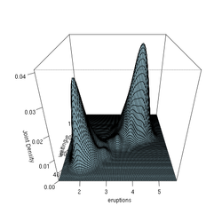
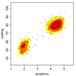Old Faithful Geyser data kernel density estimate with plug-in bandwidth matrix.

The ks package^[12] in R implements the plug-in and smoothed cross validation selectors (amongst others). This dataset (included in the base distribution of R) contains 272 records with two measurements each: the duration time of an eruprion (minutes) and the waiting time until the next eruption (minutes) of the Old Faithful Geyser in Yellowstone National Park, USA.

The code fragment computes the kernel density estimate with the plug-in bandwidth matrix $\hat{\bold{H}}_\operatorname{PI} = \begin{bmatrix}0.052 & 0.510 \\ 0.510 & 8.882\end{bmatrix}.$ Again, the coloured contours correspond to the smallest region which contains the respective probability mass: red = 25%, orange + red = 50%, yellow + orange + red = 75%. To compute the SCV selector, Hpi is replaced with Hscv. This is not displayed here since it is mostly similar to the plug-in estimate for this example.

library(ks)
data(faithful)
H <- Hpi(x=faithful)
fhat <- kde(x=faithful, H=H)
plot(fhat, display="filled.contour2")
points(faithful, cex=0.5, pch=16)

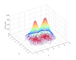
Density estimation in R with a diagonal bandwidth matrix

Old Faithful Geyser data kernel density estimate with diagonal bandwidth matrix.

This example is again based on the Old Faithful Geyser, but this time we use the R np package that employs automatic (data-driven) bandwidth selection for a diagonal bandwidth matrix; see the np vignette for an introduction to the np package. The figure below shows the joint density estimate using a second order Gaussian kernel.

R script for the example

The following commands of the R programming language use the npudens() function to deliver optimal smoothing and to create the figure given above. These commands can be entered at the command prompt by using cut and paste.

 library(np)
 library(datasets)
 data(faithful)
 f <- npudens(~eruptions+waiting,data=faithful)
 plot(f,view="fixed",neval=100,phi=30,main="",xtrim=-0.2)

Density estimation in Matlab with a diagonal bandwidth matrix

Kernel density estimate with diagonal bandwidth for synthetic normal mixture data.

We consider estimating the density of the Gaussian mixture (4π)⁻¹ exp(−¹⁄₂ (x₁² + x₂²)) + (4π)⁻¹ exp(−¹⁄₂ ((x₁ - 3.5)² + x₂²)), from 500 randomly generated points. We employ the Matlab routine for 2-dimensional data. The routine is an automatic bandwidth selection method specifically designed for a second order Gaussian kernel ^[13]. The figure shows the joint density estimate that results from using the automatically selected bandwidth.

Matlab script for the example

Type the following commands in Matlab after downloading and saving the function kde2d.m in the current directory.

 clear all  
 % generate synthetic data
data=[randn(500,2);
      randn(500,1)+3.5, randn(500,1);];
  % call the routine, which has been saved in the current directory 
    [bandwidth,density,X,Y]=kde2d(data);
  % plot the data and the density estimate
    contour3(X,Y,density,50), hold on
    plot(data(:,1),data(:,2),'r.','MarkerSize',5)

Alternative optimality criteria

The MISE is the expected integrated L₂ distance between the density estimate and the true density function f. It is the most widely used, mostly due to its tractability and most software implement MISE-based bandwidth selectors. There are alternative optimality criteria, which attempt to cover cases where MISE is not an appropriate measure.^[3]:34-37,78 The equivalent L₁ measure, Mean Integrated Absolute Error, is

$\operatorname{MIAE} (\bold{H}) = \operatorname{E}\, \int |\hat{f}_\bold{H} (\bold{x}) - f(\bold{x})| \, d\bold{x}.$

Its mathematical analysis is considerably more difficult than the MISE ones. In practise, the gain appears not to be significant.^[14] The L_∞ norm is the Mean Uniform Absolute Error

$\operatorname{MUAE} (\bold{H}) = \operatorname{E}\, \operatorname{sup}_{\bold{x}} |\hat{f}_\bold{H} (\bold{x}) - f(\bold{x})|.$

which has been investigated only briefly.^[15] Likelihood error criteria include those based on the Mean Kullback-Leibler distance

$\operatorname{MKL} (\bold{H}) = \int f(\bold{x}) \, \operatorname{log} [f(\bold{x})] \, d\bold{x} - \operatorname{E} \int f(\bold{x}) \, \operatorname{log} [\hat{f}(\bold{x};\bold{H})] \, d\bold{x}$

and the Mean Hellinger distance

$\operatorname{MH} (\bold{H}) = \operatorname{E} \int (\hat{f}_\bold{H} (\bold{x})^{1/2} - f(\bold{x})^{1/2})^2 \, d\bold{x} .$

The KL can be estimated using a cross-validation method, although KL cross-validation selectors can be sub-optimal even if it remains consistent for bounded density functions.^[16] MH selectors have been briefly examined in the literature.^[17]

All these optimality criteria are distance based measures, and do not always correspond to more intuitive notions of closeness, so more visual criteria have been developed in response to this concern.^[18]

References

1. ^ Rosenblatt, M. (1956). "Remarks on some nonparametric estimates of a density function". Annals of Mathematical Statistics 27: 832–837. doi:10.1214/aoms/1177728190. 
2. ^ Parzen, E. (1962). "On estimation of a probability density function and mode". Annals of Mathematical Statistics 33: 1065–1076. doi:10.1214/aoms/1177704472. 
3. ^ ^{a b} Simonoff, J.S. (1996). Smoothing Methods in Statistics. Springer. ISBN 0387947167. 
4. ^ Silverman, B.W. (1986). Density Estimation for Statistics and Data Analysis. Chapman & Hall/CRC. pp. 7–11. ISBN 0412246201. 
5. ^ ^{a b c d} Wand, M.P; Jones, M.C. (1995). Kernel Smoothing. London: Chapman & Hall/CRC. ISBN 0412552701. 
6. ^ Wand, M.P.; Jones, M.C. (1993). "Comparison of smoothing parameterizations in bivariate kernel density estimation". Journal of the American Statistical Association 88: 520–528. http://www.jstor.org/stable/2290332. 
7. ^ Duong, T.; Hazelton, M.L. (2003). "Plug-in bandwidth matrices for bivariate kernel density estimation". Journal of Nonparametric Statistics 15: 17–30. doi:10.1080/10485250306039. 
8. ^ Wand, M.P.; Jones, M.C. (1994). "Multivariate plug-in bandwidth selection". Computational Statistics 9: 97–177. 
9. ^ ^{a b c} Duong, T.; Hazelton, M.L. (2005). "Cross validation bandwidth matrices for multivariate kernel density estimation". Scandinavian Journal of Statistics 32: 485–506. doi:10.1111/j.1467-9469.2005.00445.x. 
10. ^ Hall, P.; Marron, J.; Park, B. (1992). "Smoothed cross-validation". Probability Theory and Related Fields 92: 1–20. doi:10.1007/BF01205233. 
11. ^ Duong, T.; Hazelton, M.L. (2005). "Convergence rates for unconstrained bandwidth matrix selectors in multivariate kernel density estimation". Journal of Multivariate Analysis 93: 417–433. doi:10.1016/j.jmva.2004.04.004. 
12. ^ Duong, T. (2007). "ks: Kernel density estimation and kernel discriminant analysis in R". Journal of Statistical Software 21(7). http://www.jstatsoft.org/v21/i07. 
13. ^ Botev, Z.I.; Grotowski, J.F.; Kroese, D.P. (2010). "Kernel density estimation via diffusion". Annals of Statistics 38 (5): 2916–2957. doi:10.1214/10-AOS799. 
14. ^ Hall, P.; Wand, M.P. (1988). "Minimizing L₁ distance in nonparametric density estimation". Journal of Multivariate Analysis 26: 59–88. doi:10.1016/0047-259X(88)90073-5. 
15. ^ Cao, R.; Cuevas, A.; Manteiga, W.G. (1994). "A comparative study of several smoothing methods in density estimation". Computational Statistics and Data Analysis 17: 153–176. doi:10.1016/0167-9473(92)00066-Z. 
16. ^ Hall, P. (1989). "On Kullback-Leibler loss and density estimation". Annals of Statistics 15: 589–605. doi:10.1214/aos/1176350606. 
17. ^ Ahmad, I.A.; Mugdadi, A.R. (2006). "Weighted Hellinger distance as an error criterion for bandwidth selection in kernel estimation". Journal of Nonparametric Statistics 18: 215–226. doi:10.1080/10485250600712008. 
18. ^ Marron, J.S.; Tsybakov, A. (1996). "Visual error criteria for qualitative smoothing". Journal of the American Statistical Association 90: 499–507. http://www.jstor.org/stable/2291060. 

External links

• www.mvstat.net/tduong/research A collection of peer-reviewed articles of the mathematical details of multivariate kernel density estimation and their bandwidth selectors.
• libagf A C++ library for multivariate, variable bandwidth kernel density estimation.

See also

• Kernel density estimation – univariate kernel density estimation.
• Variable kernel density estimation – estimation of multivariate densities using the kernel with variable bandwidth