Lagrange multiplier

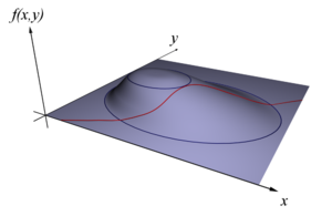Figure 1: Find x and y to maximize f(x,y) subject to a constraint (shown in red) g(x,y) = c.

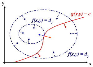Figure 2: Contour map of Figure 1. The red line shows the constraint g(x,y) = c. The blue lines are contours of f(x,y). The point where the red line tangentially touches a blue contour is our solution.

In mathematical optimization, the method of Lagrange multipliers (named after Joseph Louis Lagrange) provides a strategy for finding the maxima and minima of a function subject to constraints.

For instance (see Figure 1), consider the optimization problem

maximize $f(x, y) \,$

subject to $g(x, y) = c.\,$

We introduce a new variable (λ) called a Lagrange multiplier, and study the Lagrange function defined by

$\Lambda(x,y,\lambda) = f(x,y) + \lambda \cdot \Big(g(x,y)-c\Big),$

where the λ may be either positive or negative. If f(x,y) is a maximum for the original constrained problem, then there exists λ such that (x,y,λ) is a stationary point for the Lagrange function (stationary points are those points where the partial derivatives of Λ are zero). However, not all stationary points yield a solution of the original problem. Thus, the method of Lagrange multipliers yields a necessary condition for optimality in constrained problems.^{[1][2][3][4][5]}

Introduction

Consider the two-dimensional problem introduced above:

maximize $f(x, y) \,$

subject to $g(x, y) = c. \,$

We can visualize contours of f given by

$f(x, y)=d \,$

for various values of d, and the contour of g given by g(x,y) = c.

Suppose we walk along the contour line with g = c. In general the contour lines of f and g may be distinct, so following the contour line for g = c one could intersect with or cross the contour lines of f. This is equivalent to saying that while moving along the contour line for g = c the value of f can vary. Only when the contour line for g = c meets contour lines of f tangentially, do we not increase or decrease the value of f — that is, when the contour lines touch but do not cross.

The contour lines of f and g touch when the tangent vectors of the contour lines are parallel. Since the gradient of a function is perpendicular to the contour lines, this is the same as saying that the gradients of f and g are parallel. Thus we want points (x,y) where g(x,y) = c and

$\nabla_{x,y} f = - \lambda \nabla_{x,y} g$,

where

$\nabla_{x,y} f= \left( \frac{\partial f}{\partial x}, \frac{\partial f}{\partial y} \right)$

and

$\nabla_{x,y} g= \left( \frac{\partial g}{\partial x}, \frac{\partial g}{\partial y} \right)$

are the respective gradients. The constant λ is required because although the two gradient vectors are parallel, the magnitudes of the gradient vectors are generally not equal.

To incorporate these conditions into one equation, we introduce an auxiliary function

$\Lambda(x,y,\lambda) = f(x,y) + \lambda \cdot \Big(g(x,y)-c\Big),$

and solve

$\nabla_{x,y,\lambda} \Lambda(x , y, \lambda)=0.$

This is the method of Lagrange multipliers. Note that $\nabla_{\lambda} \Lambda(x , y, \lambda)=0$ implies g(x,y) = c.

Not necessarily extrema

The constrained extrema of f are critical points of the Lagrangian Λ, but they are not local extrema of Λ (see Example 2 below).

One may reformulate the Lagrangian as a Hamiltonian, in which case the solutions are local minima for the Hamiltonian. This is done in optimal control theory, in the form of Pontryagin's minimum principle.

The fact that solutions of the Lagrangian are not necessarily extrema also poses difficulties for numerical optimization. This can be addressed by computing the magnitude of the gradient, as the zeros of the magnitude are necessarily local minima, as illustrated in the numerical optimization example.

Handling multiple constraints

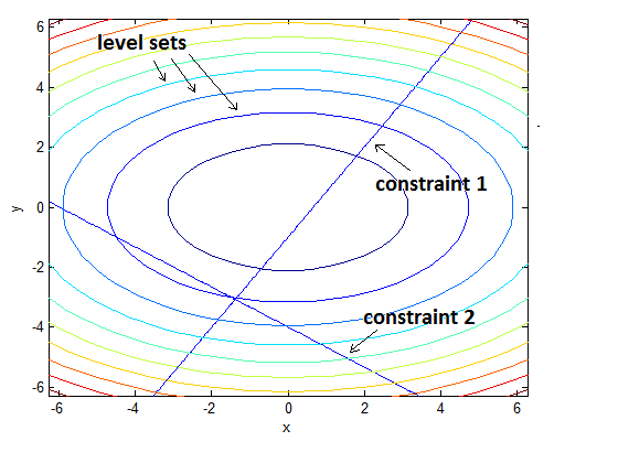
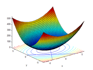A paraboloid, some of its level sets (aka contour lines) and 2 line constraints.

Zooming in on the levels sets and constraints, we see that the two constraint lines intersect to form a "joint" constraint that is a point. Since there is only one point to analyze, the corresponding point on the paraboloid is automatically a minimum and maximum. Yet the simplified reasoning presented in sections above seems to fail because the level set definitely appears to "cross" the point and at the same time its gradient is not parallel to the gradients of either constraint. This shows we must refine our explanation of the method to handle the kinds of constraints that are formed when we have more than one constraint acting at once.

The method of Lagrange multipliers can also accommodate multiple constraints. To see how this is done, we need to reexamine the problem in a slightly different manner because the concept of “crossing” discussed above becomes rapidly unclear when we consider the types of constraints that are created when we have more than one constraint acting together.

As an example, consider a paraboloid with a constraint that is a single point (as might be created if we had 2 line constraints that intersect). The level set (i.e., contour line) clearly appears to “cross” that point and its gradient is clearly not parallel to the gradients of either of the two line constraints. Yet, it is obviously a maximum and a minimum because there is only one point on the paraboloid that meets the constraint.

While this example seems a bit odd, it is easy to understand and is representative of the sort of “effective” constraint that appears quite often when we deal with multiple constraints intersecting. Thus, we take a slightly different approach below to explain and derive the Lagrange Multipliers method with any number of constraints.

Throughout this section, the independent variables will be denoted by $x_1,x_2,\ldots ,x_N$ and, as a group, we will denote them as $p=\left( x_1,x_2,\ldots ,x_N \right)$. Also, the function being analyzed will be denoted by $f\left( p \right)$ and the constraints will be represented by the equations $g_{1}\left( p \right) = 0,g_{2}\left( p \right) = 0,\,\,\ldots ,g_{M}\left( p \right) = 0$.

The basic idea remains essentially the same: if we consider only the points that satisfy the constraints (i.e. are in the constraints), then a point $\left( p,f\left( p \right) \right)$ is a stationary point (i.e. a point in a “flat” region) of f if and only if the constraints at that point do not allow movement in a direction where f changes value.

Once we have located the stationary points, we need to do further tests to see if we have found a minimum, a maximum or just a stationary point that is neither.

We start by considering the level set of f at $\left( p,f\left( p \right) \right)$. The set of vectors $\left\{ v_{L} \right\}$ containing the directions in which we can move and still remain in the same level set are the directions where the value of f does not change (i.e. the change equals zero). Thus, for every vector v in $\left\{ v_{L} \right\}$, the following relation must hold:

$\Delta f=\frac{df}{dx_{1}}v_{x_{1}}+\frac{df}{dx_{2}}v_{x_{2}}+\,\,\,\cdots \,\,\,+\frac{df}{dx_{N}}v_{x_{N}}=0$

where the notation $v_{x_{K}}$ above means the x_K-component of the vector v. The equation above can be rewritten in a more compact geometric form that helps our intuition:

$\begin{matrix} \underbrace{\begin{matrix} \left[ \begin{matrix} \frac{df}{dx_{1}} \\ \frac{df}{dx_{2}} \\ \vdots \\ \frac{df}{dx_{N}} \\ \end{matrix} \right] \\ {} \\ \end{matrix}}_{\nabla f} & \centerdot & \underbrace{\begin{matrix} \left[ \begin{matrix} v_{x_{1}} \\ v_{x_{2}} \\ \vdots \\ v_{x_{N}} \\ \end{matrix} \right] \\ {} \\ \end{matrix}}_{v} & =\,\,0 \\ \end{matrix}\,\,\,\,\,\,\,\,\,\,\,\,\Rightarrow \,\,\,\,\,\,\,\,\nabla f\,\,\,\centerdot \,\,\,\,v\,\,=\,\,\,0$

This makes it clear that if we are at p, then all directions from this point that do not change the value of f must be perpendicular to $\nabla f\left( p \right)$ (the gradient of f at p).

Now let us consider the effect of the constraints. Each constraint limits the directions that we can move from a particular point and still satisfy the constraint. We can use the same procedure, to look for the set of vectors $\left\{ v_{C} \right\}$ containing the directions in which we can move and still satisfy the constraint. As above, for every vector v in $\left\{ v_{C} \right\}$, the following relation must hold:

$\Delta g=\frac{dg}{dx_{1}}v_{x_{1}}+\frac{dg}{dx_{2}}v_{x_{2}}+\,\,\,\cdots \,\,\,+\frac{dg}{dx_{N}}v_{x_{N}}=0\,\,\,\,\,\,\,\,\,\,\,\,\,\Rightarrow \,\,\,\,\,\,\,\,\,\,\,\nabla g\,\,\centerdot \,\,\,v\,\,=\,\,\,0$

From this, we see that at point p, all directions from this point that will still satisfy this constraint must be perpendicular to $\nabla g\left( p \right)$ .

Now we are ready to refine our idea further and complete the method: a point on f is a constrained stationary point if and only if the direction that changes f violates at least one of the constraints. (We can see that this is true because if a direction that changes f did not violate any constraints, then there would a “legal” point nearby with a higher or lower value for f and the current point would then not be a stationary point.)

Single constraint revisited

For a single constraint, we use the statement above to say that at stationary points the direction that changes f is in the same direction that violates the constraint. To determine if two vectors are in the same direction, we note that if two vectors start from the same point and are “in the same direction”, then one vector can always “reach” the other by changing its length and/or flipping to point the opposite way along the same direction line. In this way, we can succinctly state that two vectors point in the same direction if and only if one of them can be multiplied by some real number such that they become equal to the other. So, for our purposes, we require that:

$\nabla f\left( p \right)=\lambda \, \nabla g\left( p \right) \qquad \Rightarrow \qquad \nabla f\left( p \right)-\lambda \, \nabla g\left( p \right)\,\,=\,\,0$

If we now add another simultaneous equation to guarantee that we only perform this test when we are at a point that satisfies the constraint, we end up with 2 simultaneous equations that when solved, identify all constrained stationary points:

$\begin{cases} g\left( p \right)=0 & \text{means point satisfies constraint} \\ \nabla f\left( p \right)-\lambda \, \nabla g\left( p \right) = 0 & \text{means point is a stationary point} \end{cases}$

Note that the above is a succinct way of writing the equations. Fully expanded, there are N + 1 simultaneous equations that need to be solved for the N + 1 variables which are λ and $x_1,\ x_2, \ldots, x_N$:

$\begin{align} g\left( x_1, x_2, \ldots , x_N \right) & =0 \\ \frac{df}{dx_1}\left( x_1, x_2, \ldots, x_N \right) - \lambda \frac{dg}{dx_1}\left( x_1, x_2,\ldots , x_N \right) & = 0 \\ \frac{df}{dx_2}\left( x_1, x_2, \ldots , x_N \right) - \lambda \frac{dg}{dx_2}\left( x_1, x_2, \ldots, x_N \right) & = 0 \\ & {}\ \ \vdots \\ \frac{df}{dx_N}\left( x_1, x_2, \ldots x_N \right) - \lambda \frac{dg}{dx_N}\left( x_1, x_2, \ldots, x_N \right) & = 0 \end{align}$

Multiple constraints

For more than one constraint, the same reasoning applies. If there is more than one constraint active together, each constraint contributes a direction that will violate it. Together, these “violation directions” form a “violation space”, where infinitesimal movement in any direction within the space will violate one or more constraints. Thus, to satisfy multiple constraints we can state (using this new terminology) that at the stationary points, the direction that changes f is in the “violation space” created by the constraints acting jointly.

The violation space created by the constraints consists of all points that can be reached by adding any combination of scaled and/or flipped versions of the individual violation direction vectors. In other words, all the points that are “reachable” when we use the individual violation directions as the basis of the space. Thus, we can succinctly state that v is in the space defined by $b_1, b_2, \ldots ,b_M$ if and only if there exists a set of “multipliers” $\lambda_1, \lambda_2, \ldots , \lambda_M$ such that:

$\sum\limits_{k=1}^M \lambda_k b_k = v$

which for our purposes, translates to stating that the direction that changes f at p is in the “violation space” defined by the constraints $g_1,g_2, \ldots, g_M$ if and only if:

$\sum_{k=1}^M \lambda_k \nabla g_k (p) = \nabla f(p) \quad \Rightarrow \quad \nabla f(p) - \sum_{k=1}^M {\lambda_k \nabla g_k (p)} = 0$

As before, we now add simultaneous equation to guarantee that we only perform this test when we are at a point that satisfies every constraint, we end up with simultaneous equations that when solved, identify all constrained stationary points:

$\begin{matrix} \begin{align} g_1(p) & = 0 \\ g_2(p)& =0 \\ & \ \ \vdots \\ g_M(p) &= 0 \\ & \\ \nabla f(p) - \sum_{k=1}^M {\lambda_k \, \nabla g_k (p)} & = 0 \\ \end{align} & \begin{align} & \text{these mean the point satisfies all constraints} \\ & \\ & \\ & \\ & \\ & \text{this means the point is a stationary point} \\ \end{align} \\ \end{matrix}$

The method is complete now (from the standpoint of solving the problem of finding stationary points) but as mathematicians delight in doing, these equations can be further condensed into an even more elegant and succinct form. Lagrange must have cleverly noticed that the equations above look like partial derivatives of some larger scalar function L that takes all the $x_1, x_2, \ldots, x_N$ and all the $\lambda _1, \lambda_2, \ldots, \lambda _M$ as inputs. Next, he might then have noticed that setting every equation equal to zero is exactly what one would have to do to solve for the unconstrained stationary points of that larger function. Finally, he showed that a larger function L with partial derivatives that are exactly the ones we require can be constructed very simply as below:

$\begin{align} & {} \quad L\left( x_1, x_2, \ldots , x_N, \lambda_1, \lambda_2, \ldots, \lambda _M \right) \\ & = f\left( x_1, x_2, \ldots, x_N \right) - \sum\limits_{k=1}^M {\lambda_k g_k\left( x_1, x_2, \ldots , x_N \right)} \end{align}$

Solving the equation above for its unconstrained stationary points generates exactly the same stationary points as solving for the constrained stationary points of f under the constraints $g_1,g_2, \ldots, g_M$.

In Lagrange’s honor, the function above is called a Lagrangian, the scalars $\lambda_1, \lambda_2, \ldots, \lambda_M$ are called Lagrange Multipliers and this optimization method itself is called The Method of Lagrange Multipliers.

The method of Lagrange multipliers is generalized by the Karush–Kuhn–Tucker conditions, which can also take into account inequality constraints of the form h(x) ≤ c.

Interpretation of the Lagrange multipliers

Often the Lagrange multipliers have an interpretation as some quantity of interest. To see why this might be the case, observe that:

$\frac{\partial L}{\partial {g_k}} = \lambda_k.$

So, λ_k is the rate of change of the quantity being optimized as a function of the constraint variable. As examples, in Lagrangian mechanics the equations of motion are derived by finding stationary points of the action, the time integral of the difference between kinetic and potential energy. Thus, the force on a particle due to a scalar potential, $F=-\nabla V$, can be interpreted as a Lagrange multiplier determining the change in action (transfer of potential to kinetic energy) following a variation in the particle's constrained trajectory. In economics, the optimal profit to a player is calculated subject to a constrained space of actions, where a Lagrange multiplier is the increase in the value of the objective function due to the relaxation of a given constraint (e.g. through an increase in income or bribery or other means) – the marginal cost of a constraint, called the shadow price.

In control theory this is formulated instead as costate equations.

Examples

Example 1

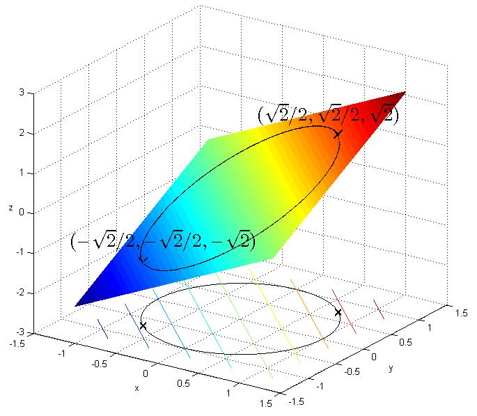
Fig. 3. Illustration of the constrained optimization problem

Suppose one wishes to maximize f(x,y) = x + y subject to the constraint x² + y² = 1. The feasible set is the unit circle, and the level sets of f are diagonal lines (with slope -1), so one can see graphically that the maximum occurs at $(\sqrt{2}/2,\sqrt{2}/2)$, and the minimum occurs at $(-\sqrt{2}/2,-\sqrt{2}/2)$.

Formally, set g(x,y) − c = x² + y² − 1, and

Λ(x,y,λ) = f(x,y) + λ(g(x,y) − c) = x + y + λ(x² + y² − 1)

Set the derivative dΛ = 0, which yields the system of equations:

$\begin{align} \frac{\partial \Lambda}{\partial x} &= 1 + 2 \lambda x &&= 0, \qquad \text{(i)} \\ \frac{\partial \Lambda}{\partial y} &= 1 + 2 \lambda y &&= 0, \qquad \text{(ii)} \\ \frac{\partial \Lambda}{\partial \lambda} &= x^2 + y^2 - 1 &&= 0, \qquad \text{(iii)} \end{align}$

As always, the $\partial \lambda$ equation ((iii) here) is the original constraint.

Combining the first two equations yields x = y (explicitly, $\lambda \neq 0$, otherwise (i) yields 1 = 0, so one has x = − 1 / (2λ) = y).

Substituting into (iii) yields 2x² = 1, so $x=y=\pm \sqrt{2}/2$ and $\lambda = \mp \sqrt{2}/2$, showing the stationary points are $(\sqrt{2}/2,\sqrt{2}/2)$ and $(-\sqrt{2}/2,-\sqrt{2}/2)$. Evaluating the objective function f on these yields

$f(\sqrt{2}/2,\sqrt{2}/2)=\sqrt{2}\mbox{ and } f(-\sqrt{2}/2, -\sqrt{2}/2)=-\sqrt{2},$

thus the maximum is $\sqrt{2}$, which is attained at $(\sqrt{2}/2,\sqrt{2}/2)$, and the minimum is $-\sqrt{2}$, which is attained at $(-\sqrt{2}/2,-\sqrt{2}/2)$.

Example 2

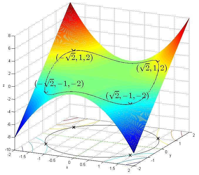
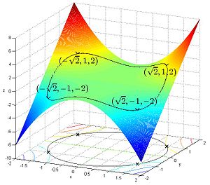Fig. 4. Illustration of the constrained optimization problem

Suppose one wants to find the maximum values of

$f(x, y) = x^2 y \,$

with the condition that the x and y coordinates lie on the circle around the origin with radius √3, that is, subject to the constraint

$g(x,y) = x^2 + y^2 = 3. \,$

As there is just a single constraint, we will use only one multiplier, say λ.

The constraint g(x, y)-3 is identically zero on the circle of radius √3. So any multiple of g(x, y)-3 may be added to f(x, y) leaving f(x, y) unchanged in the region of interest (above the circle where our original constraint is satisfied). Let

$\Lambda(x, y, \lambda) = f(x,y) + \lambda (g(x, y)-3) = x^2y + \lambda (x^2 + y^2 - 3). \,$

The critical values of Λ occur where its gradient is zero. The partial derivatives are

$\begin{align} \frac{\partial \Lambda}{\partial x} &= 2 x y + 2 \lambda x &&= 0, \qquad \text{(i)} \\ \frac{\partial \Lambda}{\partial y} &= x^2 + 2 \lambda y &&= 0, \qquad \text{(ii)} \\ \frac{\partial \Lambda}{\partial \lambda} &= x^2 + y^2 - 3 &&= 0. \qquad \text{(iii)} \end{align}$

Equation (iii) is just the original constraint. Equation (i) implies x = 0 or λ = −y. In the first case, if x = 0 then we must have $y = \pm \sqrt{3}$ by (iii) and then by (ii) λ = 0. In the second case, if λ = −y and substituting into equation (ii) we have that,

$x^2 - 2y^2 = 0. \,$

Then x² = 2y². Substituting into equation (iii) and solving for y gives this value of y:

$y = \pm 1. \,$

Thus there are six critical points:

$(\sqrt{2},1); \quad (-\sqrt{2},1); \quad (\sqrt{2},-1); \quad (-\sqrt{2},-1); \quad (0,\sqrt{3}); \quad (0,-\sqrt{3}).$

Evaluating the objective at these points, we find

$f(\pm\sqrt{2},1) = 2; \quad f(\pm\sqrt{2},-1) = -2; \quad f(0,\pm \sqrt{3})=0.$

Therefore, the objective function attains the global maximum (subject to the constraints) at $(\pm\sqrt{2},1)$ and the global minimum at $(\pm\sqrt{2},-1).$ The point $(0,\sqrt{3})$ is a local minimum and $(0,-\sqrt{3})$ is a local maximum, as may be determined by consideration of the Hessian matrix of Λ.

Note that while $(\sqrt{2}, 1, -1)$ is a critical point of Λ, it is not a local extremum. We have $\Lambda(\sqrt{2} + \epsilon, 1, -1 + \delta) = 2 + \delta(\epsilon^2 + (2\sqrt{2})\epsilon)$. Given any neighborhood of $(\sqrt{2}, 1, -1)$, we can choose a small positive $\epsilon$ and a small δ of either sign to get Λ values both greater and less than 2.

Example: entropy

Suppose we wish to find the discrete probability distribution on the points $\{x_1, x_2, \ldots, x_n\}$ with maximal information entropy. This is the same as saying that we wish to find the least biased probability distribution on the points $\{x_1, x_2, \ldots, x_n\}$. In other words, we wish to maximize the Shannon entropy equation:

$f(p_1,p_2,\ldots,p_n) = -\sum_{j=1}^n p_j\log_2 p_j.$

For this to be a probability distribution the sum of the probabilities p_i at each point x_i must equal 1, so our constraint is $g(\vec{p})$ = 1:

$g(p_1,p_2,\ldots,p_n)=\sum_{j=1}^n p_j.$

We use Lagrange multipliers to find the point of maximum entropy, $\vec{p}^{\,*}$, across all discrete probability distributions $\vec{p}$ on $\{x_1,x_2, \ldots, x_n\}$. We require that:

$\left.\frac{\partial}{\partial \vec{p}}(f+\lambda (g-1))\right|_{\vec{p}=\vec{p}^{\,*}}=0,$

which gives a system of n equations, $k ={1,\ldots,n}$, such that:

$\left.\frac{\partial}{\partial p_k}\left(-\sum_{j=1}^n p_j \log_2 p_j + \lambda \left(\sum_{j=1}^n p_j - 1\right) \right)\right|_{p_k=p^*_k} = 0.$

Carrying out the differentiation of these n equations, we get

$-\left(\frac{1}{\ln 2}+\log_2 p^*_k \right) + \lambda = 0.$

This shows that all $p^*_k$ are equal (because they depend on λ only). By using the constraint ∑_j p_j = 1, we find

$p^*_k = \frac{1}{n}.$

Hence, the uniform distribution is the distribution with the greatest entropy, among distributions on n points.

Example: numerical optimization

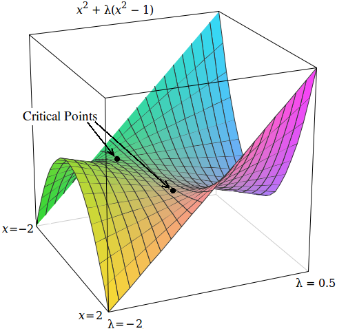
Lagrange multipliers cause the critical points to occur at saddle points.

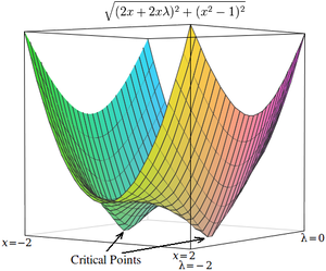The magnitude of the gradient can be used to force the critical points to occur at local minima.

With Lagrange multipliers, the critical points occur at saddle points, rather than at local maxima (or minima). Unfortunately, many numerical optimization techniques, such as hill climbing, gradient descent, some of the quasi-Newton methods, among others, are designed to find local maxima (or minima) and not saddle points. For this reason, one must either modify the formulation to ensure that it's a minimization problem (for example, by extremizing the square of the gradient of the Lagrangian as below), or else use an optimization technique that finds stationary points (such as Newton's method without an extremum seeking line search) and not necessarily extrema.

As a simple example, consider the problem of finding the value of x that minimizes f(x) = x², constrained such that x² = 1. (This problem is somewhat pathological because there are only two values that satisfy this constraint, but it is useful for illustration purposes because the corresponding unconstrained function can be visualized in three dimensions.)

Using Lagrange multipliers, this problem can be converted into an unconstrained optimization problem:

Λ(x,λ) = x² + λ(x² − 1)

The two critical points occur at saddle points where x = 1 and x = − 1.

In order to solve this problem with a numerical optimization technique, we must first transform this problem such that the critical points occur at local minima. This is done by computing the magnitude of the gradient of the unconstrained optimization problem.

First, we compute the partial derivative of the unconstrained problem with respect to each variable:

$\frac{\partial \Lambda}{\partial x}=2x+2x\lambda$

$\frac{\partial \Lambda}{\partial \lambda}=x^2-1$

If the target function is not easily differentiable, the differential with respect to each variable can be approximated as

$\frac{\partial \Lambda}{\partial x}\approx\frac{\Lambda(x+\epsilon,\lambda)-\Lambda(x,\lambda)}{\epsilon}$,

$\frac{\partial \Lambda}{\partial \lambda}\approx\frac{\Lambda(x,\lambda+\epsilon)-\Lambda(x,\lambda)}{\epsilon}$,

where $\epsilon$ is a small value.

Next, we compute the magnitude of the gradient, which is the square root of the sum of the squares of the partial derivatives:

$h(x,\lambda)=\sqrt{(2x+2x\lambda)^2+(x^2-1)^2}\approx\sqrt{\left(\frac{\Lambda(x+\epsilon,\lambda)-\Lambda(x,\lambda)}{\epsilon}\right)^2+\left(\frac{\Lambda(x,\lambda+\epsilon)-\Lambda(x,\lambda)}{\epsilon}\right)^2}$

(Since magnitude is always non-negative, optimizing over the squared-magnitude is equivalent to optimizing over the magnitude. Thus, the ``square root" may be omitted from these equations with no expected difference in the results of optimization.)

The critical points of h occur at x = 1 and x = − 1, just as in Λ. Unlike the critical points in Λ, however, the critical points in h occur at local minima, so numerical optimization techniques can be used to find them.

Applications

Economics

Constrained optimization plays a central role in economics. For example, the choice problem for a consumer is represented as one of maximizing a utility function subject to a budget constraint. The Lagrange multiplier has an economic interpretation as the shadow price associated with the constraint, in this example the marginal utility of income.

Control theory

In optimal control theory, the Lagrange multipliers are interpreted as costate variables, and Lagrange multipliers are reformulated as the minimization of the Hamiltonian, in Pontryagin's minimum principle.

See also

• Karush–Kuhn–Tucker conditions: generalization of the method of Lagrange multipliers.
• Lagrange multipliers on Banach spaces: another generalization of the method of Lagrange multipliers.
• Dual problem
• Lagrangian relaxation

References

1. ^ Bertsekas, Dimitri P. (1999). Nonlinear Programming (Second ed.). Cambridge, MA.: Athena Scientific. ISBN 1-886529-00-0. 
2. ^ Vapnyarskii, I.B. (2001), "Lagrange multipliers", in Hazewinkel, Michiel, Encyclopaedia of Mathematics, Springer, ISBN 978-1556080104, http://eom.springer.de/L/l057190.htm .
3. ^
   • Lasdon, Leon S. (1970). Optimization theory for large systems. Macmillan series in operations research. New York: The Macmillan Company. pp. xi+523. MR337317. 
   • Lasdon, Leon S. (2002). Optimization theory for large systems (reprint of the 1970 Macmillan ed.). Mineola, New York: Dover Publications, Inc.. pp. xiii+523. MR1888251. 
4. ^ Hiriart-Urruty, Jean-Baptiste; Lemaréchal, Claude (1993). "XII Abstract duality for practitioners". Convex analysis and minimization algorithms, Volume II: Advanced theory and bundle methods. Grundlehren der Mathematischen Wissenschaften [Fundamental Principles of Mathematical Sciences]. 306. Berlin: Springer-Verlag. pp. 136–193 (and Bibliographical comments on pp. 334–335). ISBN 3-540-56852-2. 
5. ^ Lemaréchal, Claude (2001). "Lagrangian relaxation". In Michael Jünger and Denis Naddef. Computational combinatorial optimization: Papers from the Spring School held in Schloß Dagstuhl, May 15–19, 2000. Lecture Notes in Computer Science. 2241. Berlin: Springer-Verlag. pp. 112–156. doi:10.1007/3-540-45586-8_4. ISBN 3-540-42877-1. MRdoi:[http://dx.doi.org/10.1007%2F3-540-45586-8_4 10.1007/3-540-45586-8_4 1900016.[[Digital object identifier|doi]]:[http://dx.doi.org/10.1007%2F3-540-45586-8_4 10.1007/3-540-45586-8_4]]. 

External links

Exposition

• Conceptual introduction (plus a brief discussion of Lagrange multipliers in the calculus of variations as used in physics)
• Lagrange Multipliers for Quadratic Forms With Linear Constraints by Kenneth H. Carpenter

For additional text and interactive applets

• Simple explanation with an example of governments using taxes as Lagrange multipliers
• Applet
• Tutorial and applet
• Video Lecture of Lagrange Multipliers
• MIT Video Lecture on Lagrange Multipliers
• Slides accompanying Bertsekas's nonlinear optimization text, with details on Lagrange multipliers (lectures 11 and 12)
• http://eom.springer.de/L/l057190.htm