Legendre transformation

---

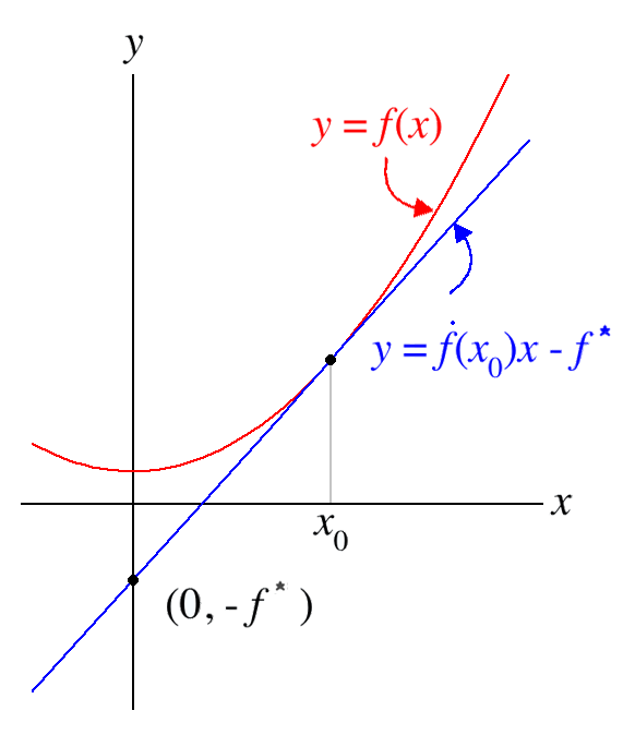
thumb|256px|right|Diagram illustrating the Legendre transformation of the function ">$f(x)$ . The function is shown in red, and the tangent line at point $(x\_0,\; f(x\_0))$ is shown in blue. The tangent line intersects the vertical axis at $(0,\; -\; f^star)$ and $f^star$ is the value of the Legendre transform $f^star(p\_0)$ , where $p\_0=dot\{f\}(x\_0)$ . Note that for any other point on the red curve, a line drawn through that point with the same slope as the blue line will have a "y"-intercept above the point $(0,\; -\; f^star)$ , showing that $f^star$ is indeed a maximum.

In mathematics, it is often desirable to express a functional relationship $f(x),$ as a different function, whose argument is the derivative of "f" , rather than "x" . If we let $p\; =\; frac\{mathrm\{d\}f\}\{mathrm\{d\}x\}$ be the argument of this new function, then this new function is written $f^star(p),$ and is called the Legendre transform of the original function, after Adrien-Marie Legendre.

The Legendre transform $f^star$ of a function $f,$ is defined as follows:

:$f^star(p)\; =\; mathrm\{max\}\_x(px-f(x)).$

The notation $max\_x$ indicates the maximization of the expression with respect to the variable $x$ while "p" is held constant. The Legendre transform is its own inverse. Like the familiar Fourier transform, the Legendre transform takes a function $f(x)$ and produces a function of a different variable $p$. However, while the Fourier transform consists of an integration with a kernel, the Legendre transform uses maximization as the transformation procedure. The transform is well behaved only if $f(x)$ is a convex function.

The Legendre transformation is an application of the duality relationship between points and lines. The functional relationship specified by "f"("x") can be represented equally well as a set of ("x", "y") points, or as a set of tangent lines specified by their slope and intercept values.

The Legendre transformation can be generalized to the Legendre-Fenchel transformation. It is commonly used in thermodynamics and in the Hamiltonian formulation of classical mechanics.

Definitions

The definition of the Legendre transform can be made more explicit. To maximize $px-f(x)$ with respect to $x$, we set its derivative equal to zero:

::$frac\{mathrm\{d\{mathrm\{d\}x\}\; left(px-f(x)\; ight)\; =\; p-\{mathrm\{d\}f(x)\; over\; mathrm\{d\}x\}\; =\; 0.\; quad\; quad\; (1),$

Thus, the expression is maximized when :$p\; =\; \{mathrm\{d\}f(x)\; over\; mathrm\{d\}x\}.\; quad\; quad\; quad\; quad\; quad\; quad\; (2)$ This is a maximum because the second derivative is negative:

:

since $f$ was assumed convex. Next we invert (2) to obtain $x$ as a function of $p$ and plug this into (1) , which gives the more useful form,

::$f^star(p)\; =\; p\; ,,\; x(p)\; -\; f(x(p)).$

This definition gives the conventional procedure for calculating the Legendre transform of $f(x)$: find $p\; =\; \{df\; over\; dx\}$, invert for $x$ and substitute into the expression $xp-f(x)$. This definition makes clear the following interpretation: the Legendre transform produces a new function, in which the independent variable $x$ is replaced by $p\; =\; \{df\; over\; dx\}$, which is the derivative of the original function with respect to $x$.

Another definition

There is a third definition of the Legendre transform: $f,$ and $f^star$ are said to be Legendre transforms of each other if their first derivatives are inverse functions of each other:

:$Df\; =\; left(\; Df^star\; ight)^\{-1\}.$

We can see this by taking derivative of $f^star$:

:$\{df^star(p)\; over\; dp\}\; =\; \{d\; over\; dp\}(xp-f(x))\; =\; x\; +\; p\; \{dx\; over\; dp\}\; -\; \{df\; over\; dx\}\; \{dx\; over\; dp\}\; =\; x.$

Combining this equation with the maximization condition results in the following pair of reciprocal equations:

:$p\; =\; \{df\; over\; dx\}(x),$

:$x\; =\; \{df^star\; over\; dp\}(p).$

We see that $Df$ and $Df^star$ are inverses, as promised. They are unique up to an additive constant which is fixed by the additional requirement that

:$f(x)\; +\; f^star(y)\; =\; x,y.$

Although in some cases (e.g. thermodynamic potentials) a non-standard requirement is used:

:$f(x)\; -\; f^star(y)\; =\; x,y.$

The standard constraint will be considered in this article unless otherwise noted. The Legendre transformation is its own inverse, and is related to integration by parts.

Applications

Thermodynamics

The strategy behind the use of Legendre transforms is to shift, from a function with one of its parameters an independent variable, to a new function with its dependence on a new variable (the partial derivative of the original function with respect to the independent variable). The new function is the difference between the original function and the product of the old and new variables. For example, while the internal energy is an explicit function of the "extensive variables", entropy, volume (and chemical composition)

:$U\; =\; U(S,V,\{N\_i\}),$

the enthalpy, the (non standard) Legendre transform of "U" with respect to −"PV"

:$H\; =\; U\; +\; PV\; ,\; =\; H(S,P,\{N\_i\}),$:$P=,\; -left(\; frac\{partial\; U\}\{partial\; V\}\; ight)\_S,$

becomes a function of the entropy and the "intensive quantity", pressure, as natural variables, and is useful when the (external) "P" is constant. The free energies (Helmholtz and Gibbs), are obtained through further Legendre transforms, by subtracting "TS" (from "U" and "H" respectively), shift dependence from the entropy "S" to its conjugate intensive variable temperature "T", and are useful when it is constant.

Hamilton-Lagrange mechanics

A Legendre transform is used in classical mechanics to derive the Hamiltonian formulation from the Lagrangian one, and conversely. While the Lagrangian is an explicit function of the positional coordinates "q"_"j" and generalized velocities d"q"_"j" /d"t" (and time), the Hamiltonian shifts the functional dependence to the positions and "momenta",defined as $p\_j=frac\{partial\; L\}\{partial\; dot\{q\}\_j\}$.Whenever $detfrac\{partial^2\; L\}\{partial\; dot\{q\}\_ipartial\; dot\{q\}\_j\}\; eq\; 0$ (in that case the Lagrangian is said to be regular) one can express the $dot\; q\_j$ as functions $dot\; q\_j=dot\; q\_j(q\_h,\; p\_k)$ and define

:$Hleft(q\_i,p\_j,t\; ight)\; =\; sum\_m\; dot\{q\}\_m\; p\_m\; -\; L(q\_i,dot\; q\_j(q\_h,\; p\_k),t)\; ,.$

Each of the two formulations has its own applicability, both in the theoretical foundations of the subject, and in practice, depending on the ease of calculation for a particular problem. The coordinates are not necessarily rectilinear, but can also be angles, etc. An optimum choice takes advantage of the actual physical symmetries.

An example - variable capacitor

As another example from physics, consider a parallel-plate capacitor whose plates can approach or recede from one another, exchanging work with external mechanical forces which maintain the plate separation — analogous to a gas in a cylinder with a piston. We want the attractive force f between the plates as a function of the variable separation x. (The two vectors point in opposite directions.) If the "charges" on the plates remain constant as they move, the force is the negative gradient of the electrostatic energy

:

However, if the "voltage" between the plates "V" is maintained constant by connection to a battery, which is a reservoir for charge at constant potential difference, the force now becomes the negative gradient of the Legendre transform

:

The two functions happen to be negatives only because of the linearity of the capacitance. Of course, for given charge, voltage and distance, the static force must be the same by either calculation since the plates cannot "know" what might be held constant as they move.

Examples

The exponential function e^"x" has "x" ln "x" − "x" as a Legendre transform since the respective first derivatives e^"x" and ln "x" are inverse to each other. This example shows that the respective domains of a function and its Legendre transform need not agree.

Similarly, the quadratic form

:

with "A" a symmetric invertible "n"-by-"n"-matrix has

:

as a Legendre transform.

Legendre transformation in one dimension

In one dimension, a Legendre transform to a function "f" : R → R with an invertible first derivative may be found using the formula

:$f^star(y)\; =\; y\; ,\; x\; -\; f(x),\; ,\; x\; =\; dot\{f\}^\{-1\}(y)$

This can be seen by integrating both sides of the defining condition restricted to one-dimension

:$dot\{f\}(x)\; =\; dot\{f\}^\{star-1\}(x)$

from "x"₀ to "x"₁, making use of the fundamental theorem of calculus on the left hand side and substituting

:$y\; =\; dot\{f\}^\{star-1\}(x)$

on the right hand side to find

:$f(x\_1)\; -\; f(x\_0)\; =\; int\_\{y\_0\}^\{y\_1\}\; y\; ,\; ddot\{f\}^star(y)\; ,\; dy$

with "f*"′("y"₀) = "x"₀, "f*"′("y"₁) = "x"₁. Using integration by parts the last integral simplifies to

:$y\_1\; ,\; dot\{f\}^star(y\_1)\; -\; y\_0\; ,\; dot\{f\}^star(y\_0)\; -\; int\_\{y\_0\}^\{y\_1\}\; dot\{f\}^star(y)\; ,\; dy=\; y\_1\; ,\; x\_1\; -\; y\_0\; ,\; x\_0\; -\; f^star(y\_1)\; +\; f^star(y\_0).$

Therefore,

:$f(x\_1)\; +\; f^star(y\_1)\; -\; y\_1\; ,\; x\_1\; =\; f(x\_0)\; +\; f^star(y\_0)\; -\; y\_0\; ,\; x\_0.$

Since the left hand side of this equation does only depend on x₁ and the right hand side only on x₀, they have to evaluate to the same constant.

:$f(x)\; +\; f^star(y)\; -\; y\; ,\; x\; =\; C,,\; x\; =\; dot\{f\}^star(y)\; =\; dot\{f\}^\{-1\}(y).$

Solving for "f*" and choosing "C" to be zero results in the above-mentioned formula.

Geometric interpretation

For a strictly convex function the Legendre-transformation can be interpreted as a mapping between the graph of the function and the family of tangents of the graph. (For a function of one variable, the tangents are well-defined at all but at most countably many points since a convex function is differentiable at all but at most countably many points.)

The equation of a line with slope "m" and y-intercept "b" is given by

:$y\; =\; mx\; +\; b,$.

For this line to be tangent to the graph of a function "f" at the point ("x"₀, "f"("x"₀)) requires

:$fleft(x\_0\; ight)\; =\; m\; x\_0\; +\; b$

and

:$m\; =\; dot\{f\}left(x\_0\; ight)$

"f"' is strictly monotone as the derivative of a strictly convex function, and the second equation can be solved for "x"₀, allowing to eliminate "x"₀ from the first giving the "y"-intercept "b" of the tangent as a function of its slope "m":

:$b\; =\; fleft(dot\{f\}^\{-1\}left(m\; ight)\; ight)\; -\; m\; cdot\; dot\{f\}^\{-1\}left(m\; ight)\; =\; -f^star(m)$

Here "f*" denotes the Legendre transform of "f".

The family of tangents of the graph of "f" is therefore (parameterized by "m") given by

:$y\; =\; mx\; -\; f^star(m)$

or, written implicitly, by the solutions of the equation

:$F(x,y,m)\; =\; y\; +\; f^star(m)\; -\; mx\; =\; 0.$

The graph of the original function can be reconstructed from this family of lines as the envelope of this family by demanding

: $\{partial\; F(x,y,m)overpartial\; m\}\; =\; dot\{f\}^star(m)\; -\; x\; =\; 0.$

Eliminating "m" from these two equations gives

: $y\; =\; x\; cdot\; dot\{f\}^\{star-1\}(x)\; -\; f^starleft(dot\{f\}^\{star-1\}(x)\; ight).$

Identifying "y" with "f"("x") and recognizing the right side of the preceding equation as the Legendre transform of "f"* we find

: $f(x)\; =\; f^\{starstar\}(x).$

Legendre transformation in more than one dimension

For a differentiable real-valued function on an open subset "U" of Rⁿ the Legendre conjugate of the pair ("U", "f") is defined to be the pair ("V", "g"), where "V" is the image of "U" under the gradient mapping D"f", and "g" is the function on "V" given by the formula

:$g(y)\; =\; leftlangle\; y,\; x\; ight\; angle\; -\; fleft(x\; ight),\; ,x\; =\; left(Df\; ight)^\{-1\}(y)$

where

:$leftlangle\; u,v\; ight\; angle\; =\; sum\_\{k=1\}^\{n\}u\_\{k\}\; cdot\; v\_\{k\}$

is the scalar product on R^"n".

Alternatively, if "X" is a real vector space and "Y" is its dual vector space, then for each point "x" of "X" and "y" of "Y", there is a natural identification of the cotangent spaces T*"X"_"x" with "Y" and T*"Y"_"y" with "X". If "f" is a real differentiable function over "X", then ∇"f" is a section of the cotangent bundle T*"X" and as such, we can construct a map from "X" to "Y". Similarly, if "g" is a real differentiable function over "Y", ∇"g" defines a map from "Y" to "X". If both maps happen to be inverses of each other, we say we have a Legendre transform.

Further properties

In the following the Legendre transform of a function "f" is denoted as "f"*.

caling properties

The Legendre transformation has the following scaling properties: For "a>0",

:$f(x)\; =\; a\; cdot\; g(x)Rightarrowf^star(p)\; =\; a\; cdot\; g^starleft(frac\{p\}\{a\}\; ight)$

:$f(x)\; =\; g(a\; cdot\; x)Rightarrowf^star(p)\; =\; g^starleft(frac\{p\}\{a\}\; ight)$

It follows that if a function is homogeneous of degree "r" then its image under the Legendre transformation is a homogeneous function of degree "s", where 1/"r" + 1/"s" = 1.

Behavior under translation

:$f(x)\; =\; g(x)\; +\; bRightarrowf^star(p)\; =\; g^star(p)\; -\; b$

:$f(x)\; =\; g(x\; +\; y)Rightarrowf^star(p)\; =\; g^star(p)\; -\; p\; cdot\; y$

Behavior under inversion

:$f(x)\; =\; g^\{-1\}(x)Rightarrowf^star(p)\; =\; -\; p\; cdot\; g^starleft(frac\{1\}\{p\}\; ight)$

Behavior under linear transformations

Let "A" be a linear transformation from Rⁿ to R^m. For any convex function "f" on Rⁿ, one has:$left(A\; f\; ight)^star\; =\; f^star\; A^star$

where "A"* is the adjoint operator of "A" defined by:$left\; langle\; Ax,\; y^star\; ight\; angle\; =\; left\; langle\; x,\; A^star\; y^star\; ight\; angle$

A closed convex function "f" is symmetric with respect to a given set "G" of orthogonal linear transformations,:$fleft(A\; x\; ight)\; =\; f(x),\; ;\; forall\; x,\; ;\; forall\; A\; in\; G$
if and only if "f"* is symmetric with respect to "G".

Infimal convolution

The infimal convolution of two functions "f" and "g" is defined as:$left(f\; star\_inf\; g\; ight)(x)\; =\; inf\; left\; \{\; f(x-y)\; +\; g(y)\; ,\; |\; ,\; y\; in\; mathbb\{R\}^n\; ight\; \}$

Let "f"₁, …, "f"_m be proper convex functions on Rⁿ. Then:$left(\; f\_1\; star\_inf\; cdots\; star\_inf\; f\_m\; ight)^star\; =\; f\_1^star\; +\; cdots\; +\; f\_m^star$

ee also

* Projective duality

References

*
*