Matsubara frequency

In thermal quantum field theory, the Matsubara frequency summation is the summation over discrete imaginary frequency. It takes the following form

$S_\eta = \frac{1}{\beta}\sum_{i\omega} g(i\omega)$,

where the imaginary frequency ω is usually taken from either of the following two sets (with $n,m\in\mathbb{Z}$):

$\omega_n=\frac{2n\pi}{\beta}$, bosonic frequencies,

$\omega_m=\frac{(2m+1)\pi}{\beta}$, fermionic frequencies.

The summation will converge if g(z=iω) tends to 0 in z→∞ limit in a manner faster than z ^{− 1}. The summation over bosonic frequencies is denoted as S_B (with η=+1), while that over fermionic frequencies is denoted as S_F (with η=-1). η marks the statistical sign.

Matsubara Frequency Summation

General Formalism

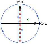Figure 1.

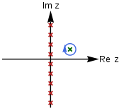Figure 2.

The trick to evaluate Matsubara frequency summation is to use a Matsubara weighting function h_η(z) that has simple poles located exactly at z = iω. The weighting functions differs from the boson case η=+1 to the fermion case η=-1. The choice of weighing function will be discussed later. With the weighting function, the summation can be replaced by a contour integral in the complex plane.

$S_\eta=\frac{1}{\beta}\sum_{i\omega} g(i\omega)=\frac{1}{2\pi i\beta}\oint g(z) h_\eta(z) dz$.

As in Fig. 1, the weighting function generates poles (red crosses) on the imaginary axis. The contour integral picks up the residue of these poles, which is equivalent to the summation.

By deformation of the contour lines to enclose the poles of g(z) (the green cross in Fig. 2), the summation can be formally accomplished by summing the residue of g(z)h_η(z) over all poles of g(z),

$S_\eta=-\frac{1}{\beta}\sum_{z_0\in g(z)\text{ poles}}\text{Res}\,g(z_0)h_\eta(z_0)$.

Note that a minus sign is produced, because the contour is deformed to enclose the poles in the clockwise direction, resulting in the negative residue.

Choice of Matsubara Weighting Function

To produce simple poles on boson frequencies z = iω_n, either of the following two types of Matsubara weighting functions can be chosen

$h_B^{(1)}(z)=\frac{\beta}{1-e^{-\beta z}}=-\beta n_B(-z)=\beta(1+n_B(z))$,

$h_B^{(2)}(z)=\frac{-\beta}{1-e^{\beta z}}=\beta n_B(z)$,

depending on which half plane the convergence is to be controlled in. $h_B^{(1)}(z)$ controls the convergence in the left half plane (Re z<0), while $h_B^{(2)}(z)$ controls the convergence in the right half plane (Re z>0). Here n_B(z) = (e^βz − 1) ^{− 1} is the Bose-Einstein distribution function.

The case is similar for fermion frequencies. There are also two types of Matsubara weighting functions that produce simple poles at z = iω_m

$h_F^{(1)}(z)=\frac{\beta}{1+e^{-\beta z}}=\beta n_F(-z)=\beta(1-n_F(z))$,

$h_F^{(2)}(z)=\frac{-\beta}{1+e^{\beta z}}=-\beta n_F(z)$.

$h_F^{(1)}(z)$ controls the convergence in the left half plane (Re z<0), while $h_F^{(2)}(z)$ controls the convergence in the right half plane (Re z>0). Here n_F(z) = (e^βz + 1) ^{− 1} is the Fermi-Dirac distribution function.

In the application to Green's function calculation, g(z) always have the structure

g(z) = G(z)e ^{− zτ},

which diverges in the left half plane given 0<τ<β. So as to control the convergence, the weighting function of the first type is always chosen $h_\eta(z)=h_\eta^{(1)}(z)$. However there is no need to control the convergence if the Matsubara summation does not diverge, in that case, any choice of the Matsubara weighting function will lead to identical results.

Table of Matsubara Frequency Summations

The following table concludes the Matsubara frequency summations for some simple rational functions g(z).

$S_\eta=\frac{1}{\beta}\sum_{i\omega}g(i\omega)$.

η=±1 marks the statistical sign.

g(iω)	Sη
(iω − ξ) − 1	− ηnη(ξ) − 1 / 2[1]
(iω − ξ) − 2	$-\eta n_\eta^\prime(\xi)=\beta n_\eta(\xi)(\eta+n_\eta(\xi))$
(iω − ξ) − n	$-\frac{\eta}{(n-1)!}\partial_\xi^{n-1} n_\eta(\xi)$
$\frac{1}{(i\omega-\xi_1)(i\omega-\xi_2)}$	$-\frac{\eta(n_\eta(\xi_1)-n_\eta(\xi_2))}{\xi_1-\xi_2}$
$\frac{1}{(i\omega-\xi_1)^2(i\omega-\xi_2)^2}$	$\frac{\eta}{(\xi_1-\xi_2)^2}\left(\frac{2(n_\eta(\xi_1)-n_\eta(\xi_2))}{\xi_1-\xi_2}-(n_\eta^\prime(\xi_1)+n_\eta^\prime(\xi_2))\right)$
$\frac{1}{(i\omega-\xi_1)^2-\xi_2^2}$	ηcη(ξ1,ξ2)
$\frac{1}{(i\omega)^2-\xi^2}$	$\eta c_\eta(0,\xi)=-\frac{1}{2\xi}(1+2\eta n_\eta(\xi))$
$\frac{(i\omega)^2}{(i\omega)^2-\xi^2}$	$-\frac{\xi}{2}(1+2\eta n_\eta(\xi))$
$\frac{1}{((i\omega)^2-\xi^2)^2}$	$-\frac{\eta}{2\xi^2}(c_\eta(0,\xi)+ n_\eta^\prime(\xi))$
$\frac{(i\omega)^2}{((i\omega)^2-\xi^2)^2}$	$\frac{\eta}{2}(c_\eta(0,\xi)- n_\eta^\prime(\xi))$
$\frac{(i\omega)^2+\xi^2}{((i\omega)^2-\xi^2)^2}$	$-\eta n_\eta^\prime(\xi)=\beta n_\eta(\xi)(\eta+n_\eta(\xi))$
$\frac{1}{((i\omega)^2-\xi_1^2)((i\omega)^2-\xi_2^2)}$	$\frac{\eta(c_\eta(0,\xi_1)-c_\eta(0,\xi_2))}{\xi_1^2-\xi_2^2}$
$\left(\frac{1}{(i\omega)^2-\xi_1^2}+\frac{1}{(i\omega)^2-\xi_2^2}\right)^2$	$\eta\left(\frac{3\xi_1^2+\xi_2^2}{2\xi_1^2(\xi_1^2-\xi_2^2)}c_\eta(0,\xi_1) - \frac{n_\eta^\prime(\xi_1)}{2\xi_1^2}\right)+(1\leftrightarrow 2)$[2]
$\left(\frac{1}{(i\omega)^2-\xi_1^2}-\frac{1}{(i\omega)^2-\xi_2^2}\right)^2$	$\eta\left(-\frac{5\xi_1^2-\xi_2^2}{2\xi_1^2(\xi_1^2-\xi_2^2)}c_\eta(0,\xi_1) - \frac{n_\eta^\prime(\xi_1)}{2\xi_1^2}\right)+(1\leftrightarrow 2)$[2]

[1] Since the summation does not converge, the result may differ by a constant upon different choice of the Matsubara weighting function.

[2] (1↔2) indicates the same expression as the before but with index 1 and 2 exchanged.

Applications in Physics

Zero Temperature Limit

In this limit $\beta\rightarrow\infty$, the Matsubara frequency summation is equivalent to the integration of imaginary frequency over imaginary axis.

$\frac{1}{\beta}\sum_{i\omega}=\int_{-i\infty}^{i\infty}\frac{\mathrm{d}(i\omega)}{2\pi}$.

Some of the integrals do not converge. They should be regularized by introducing the frequency cutoff Ω, and then subtracting the divergent part (Ω-dependent) from the integral before taking the limit of $\Omega\rightarrow\infty$. For example, the free energy is obtained by the integral of logarithm,

$\eta \lim_{\Omega\rightarrow\infty}\left[ \int_{-i\Omega}^{i\Omega}\frac{\mathrm{d}(i\omega)}{2\pi} \left(\ln(-i\omega+\xi)-\frac{\pi\xi}{2\Omega}\right)-\frac{\Omega}{\pi}(\ln\Omega-1)\right] =\left\{ \begin{array}{cc} 0 & \xi\geq0 \\ -\eta\xi & \xi<0 \end{array} \right.,$

meaning that at zero temperature, the free energy simply relates to the internal energy below the chemical potential. Also the distribution function is obtained by the following integral

$\eta \lim_{\Omega\rightarrow\infty} \int_{-i\Omega}^{i\Omega}\frac{\mathrm{d}(i\omega)}{2\pi} \left(\frac{1}{-i\omega+\xi}-\frac{\pi}{2\Omega}\right) =\left\{ \begin{array}{cc} 0 & \xi\geq0 \\ -\eta & \xi<0 \end{array} \right.,$

which shows step function behavior at zero temperature.

Green's Function Related

Time Domain

Consider a function G(τ) defined on the imaginary time interval (0,β). It can be given in terms of Fourier series,

$G(\tau)=\frac{1}{\beta}\sum_{i\omega} G(i\omega) e^{-i\omega\tau}$,

where the frequency only takes discrete values spaced by 2π/β.

The particular choice of frequency depends on the boundary condition of the function G(τ). In physics, G(τ) stands for the imaginary time representation of Green's function

$G(\tau)=-\langle \mathcal{T}_\tau \psi(\tau)\psi^*(0) \rangle$.

It satisfies periodic boundary condition G(τ+β)=G(τ) for boson field. While for fermion field the boundary condition is anti-periodic G(τ+β)=-G(τ).

Given the Green's function G(iω) in the frequency domain, its imaginary time representation G(τ) can be evaluated by Matsubara frequency summation. Depending on the boson or fermion frequencies that is to be summed over, the resulting G(τ) can be different. To distinguish, define

$G_\eta(\tau)= \begin{cases} G_B(\tau), & \mbox{if } \eta = +1 \\ G_F(\tau), & \mbox{if } \eta = -1 \end{cases}$,

with

$G_B(\tau)=\frac{1}{\beta}\sum_{i\omega_n}G(i\omega_n)e^{-i\omega_n\tau}$,

$G_F(\tau)=\frac{1}{\beta}\sum_{i\omega_m}G(i\omega_m)e^{-i\omega_m\tau}$.

Note that τ is restricted in the principal interval (0,β). The boundary condition can be used to extend G(τ) out of the principal interval. Some frequently used results are concluded in the following table.

G(iω)	Gη(τ)
(iω − ξ) − 1	− eξ(β − τ)nη(ξ)
(iω − ξ) − 2	$e^{\xi(\beta-\tau)}n_\eta(\xi)\left(\tau+\eta\beta n_\eta(\xi)\right)$
(iω − ξ) − 3	$-\frac{1}{2}e^{\xi(\beta-\tau)}n_\eta(\xi)\left(\tau^2+\eta\beta(\beta+2\tau) n_\eta(\xi)+2\beta^2n^2_\eta(\xi)\right)$
(iω − ξ1) − 1(iω − ξ2) − 1	$-\frac{e^{\xi_1(\beta-\tau)}n_\eta(\xi_1)-e^{\xi_2(\beta-\tau)}n_\eta(\xi_2)}{\xi_1-\xi_2}$
(ω2 + m2) − 1	$\frac{e^{-m\tau}}{2m}+\frac{\eta}{m}\cosh{m\tau}\;n_\eta(m)$
iω(ω2 + m2) − 1	$\frac{e^{-m\tau}}{2}-\eta\,\sinh{m\tau}\;n_\eta(m)$

Operator Switching Effect

The small imaginary time plays a critical role here. The order of the operators will change if the small imaginary time changes sign.

$\langle \psi\psi^*\rangle=\langle \mathcal{T}_\tau \psi(\tau=0^+) \psi^*(0)\rangle =-G_\eta(\tau=0^+)=-\frac{1}{\beta}\sum_{i\omega}G(i\omega)e^{-i\omega 0^+}$.

$\langle \psi^*\psi\rangle=\eta\langle \mathcal{T}_\tau \psi(\tau=0^-) \psi^*(0)\rangle =-\eta G_\eta(\tau=0^-)=-\frac{\eta}{\beta}\sum_{i\omega}G(i\omega)e^{i\omega 0^+}$

Distribution Function

The evaluation of distribution function becomes tricky because of the discontinuity of Green's function G(τ) at τ=0. To evaluate the summation

G(0) =	∑	(iω − ξ) − 1
	iω

, both choices of the weighting function are acceptable, but the results are different. This can be understood if we push G(τ) away from τ=0 a little bit, then to control the convergence, we must take $h_\eta^{(1)}(z)$ as the weighting function for G(τ = 0 ⁺ ), and $h_\eta^{(2)}(z)$ for G(τ = 0 ⁻ ).

Bosons

$G_B(\tau=0^-)=\frac{1}{\beta}\sum_{i\omega_n}\frac{e^{i\omega_n 0^+}}{i\omega_n-\xi}=-n_B(\xi)$,

$G_B(\tau=0^+)=\frac{1}{\beta}\sum_{i\omega_n}\frac{e^{-i\omega_n 0^+}}{i\omega_n-\xi}=-(n_B(\xi)+1)$.

Fermions

$G_F(\tau=0^-)=\frac{1}{\beta}\sum_{i\omega_m}\frac{e^{i\omega_m 0^+}}{i\omega_m-\xi}=n_F(\xi)$,

$G_F(\tau=0^+)=\frac{1}{\beta}\sum_{i\omega_m}\frac{e^{-i\omega_m 0^+}}{i\omega_m-\xi}=-(1-n_F(\xi))$.

Free Energy

Bosons

$\frac{1}{\beta}\sum_{i\omega_n} \ln(-i\omega_n+\xi)=\frac{1}{\beta}\ln(1-e^{-\beta\xi})$,

Fermions

$-\frac{1}{\beta}\sum_{i\omega_m} \ln(-i\omega_m+\xi)=-\frac{1}{\beta}\ln(1+e^{-\beta\xi})$.

Diagrams Evaluation

Frequently encountered diagrams are evaluated here with the single mode setting. Multiple modes problem can be approached by spectral function integral.

Fermion Self Energy

$\Sigma(i\omega_m)=-\frac{1}{\beta }\sum _{i \omega_n } \frac{1}{i \omega_m +i \omega_n -\epsilon }\frac{1}{i \omega_n -\Omega }=\frac{n_F(\epsilon )+n_B(\Omega )}{i \omega_m -\epsilon +\Omega }$.

Particle-Particle Bubble

$\Pi (i \omega_n )=\frac{1}{\beta }\sum _{i \omega_m } \frac{1}{i \omega_m +i \omega_n -\epsilon }\frac{1}{i \omega_m -\epsilon '}=-\frac{n_F(\epsilon )-n_F\left(\epsilon '\right)}{i \omega_n -\epsilon +\epsilon '}$.

Particle-Hole Bubble

$\Pi (i \omega_n )=-\frac{1}{\beta }\sum _{i \omega_m } \frac{1}{i \omega_m +i \omega_n -\epsilon }\frac{1}{-i \omega_m -\epsilon '}=\frac{1-n_F(\epsilon )-n_F\left(\epsilon '\right)}{i \omega_n -\epsilon -\epsilon '}.$

Appendix: Properties of Distribution Functions

Distribution Functions

The general notation n_η stands for either Bose (η=+1) or Fermi (η=-1) distribution function

$n_\eta(\xi)=\frac{1}{e^{\beta\xi}-\eta}$.

If necessary, the specific notations n_B and n_F are used to indicate Bose and Fermi distribution functions respectively

$n_\eta(\xi)= \begin{cases} n_B(\xi), & \mbox{if } \eta = +1 \\ n_F(\xi), & \mbox{if } \eta = -1 \end{cases}$.

Relation to hyperbolic functions

The Bose distribution function is related to hyperbolic cotangent function by

$n_B(\xi)=\frac{1}{2}\left(\mathrm{coth}\frac{\beta\xi}{2}-1\right)$.

The Fermi distribution function is related to hyperbolic tangent function by

$n_F(\xi)=\frac{1}{2}\left(1-\mathrm{tanh}\frac{\beta\xi}{2}\right)$.

Parity

Both distribution functions do not have definite parity,

n_η( − ξ) = − η − n_η(ξ).

Another formula is in terms of the c_η function

n_η( − ξ) = n_η(ξ) + 2ξc_η(0,ξ).

However their derivatives have definite parity.

Bose-Fermi Transmutation

Bose and Fermi distribution functions transmute under a shift of the variable by the fermionic frequency,

n_η(iω_m + ξ) = − n _{− η}(ξ).

However shifting by bosonic frequencies does not make any difference.

Derivatives

First order

$n_B^\prime(\xi)=-\frac{\beta}{4}\mathrm{csch}^2\frac{\beta \xi}{2}$,

$n_F^\prime(\xi)=-\frac{\beta}{4}\mathrm{sech}^2\frac{\beta \xi}{2}$.

In terms of product:

$n_\eta^\prime(\xi)= -\beta n_\eta(\xi)(1+\eta n_\eta(\xi))$.

In the zero temperature limit:

$n_\eta^\prime(\xi)=\eta\delta(\xi)$ as $\beta\rightarrow\infty$.

Second order

$n_B^{\prime\prime}(\xi)=\frac{\beta^2}{4}\mathrm{csch}^2\frac{\beta \xi}{2}\mathrm{coth}\frac{\beta \xi}{2}$,

$n_F^{\prime\prime}(\xi)=\frac{\beta^2}{4}\mathrm{sech}^2\frac{\beta \xi}{2}\mathrm{tanh}\frac{\beta \xi}{2}$.

Formula of difference

$n_\eta(a+b)-n_\eta(a-b)=-\frac{\mathrm{sinh}\beta b}{\mathrm{cosh}\beta a-\eta\,\mathrm{cosh}\beta b}$.

Case a=0

$n_B(b)-n_B(-b)=\mathrm{coth}\frac{\beta b}{2}$,

$n_F(b)-n_F(-b)=-\mathrm{tanh}\frac{\beta b}{2}$.

Case a→0

$n_B(a+b)-n_B(a-b)=\mathrm{coth}\frac{\beta b}{2}+n_B^{\prime\prime}(b)a^2+\cdots$,

$n_F(a+b)-n_F(a-b)=-\mathrm{tanh}\frac{\beta b}{2}+n_F^{\prime\prime}(b)a^2+\cdots$.

Case b→0

$n_B(a+b)-n_B(a-b)=2n_B^\prime(a)b+\cdots$,

$n_F(a+b)-n_F(a-b)=2n_F^\prime(a)b+\cdots$.

The function c_η

Definition:

$c_\eta(a,b)\equiv-\frac{n_\eta(a+b)-n_\eta(a-b)}{2b}$.

For Bose and Fermi type:

$c_B(a,b)\equiv c_+(a,b)$,

$c_F(a,b)\equiv c_-(a,b)$.

Relation to hyperbolic functions

$c_\eta(a,b)=\frac{\mathrm{sinh}\beta b}{2b(\mathrm{cosh}\beta a-\eta\,\mathrm{cosh}\beta b)}$.

It is obvious that c_F(a,b) is positive definite.

To avoid overflow in the numerical calculation, the tanh and coth functions are used

$c_B(a,b)=\frac{1}{4b}\left(\mathrm{coth}\frac{\beta(a-b)}{2} - \mathrm{coth}\frac{\beta(a+b)}{2}\right)$,

$c_F(a,b)=\frac{1}{4b}\left(\mathrm{tanh}\frac{\beta(a+b)}{2} - \mathrm{tanh}\frac{\beta(a-b)}{2}\right)$.

Case a=0

$c_B(0,b)=-\frac{1}{2b}\mathrm{coth}\frac{\beta b}{2}$,

$c_F(0,b)=\frac{1}{2b}\mathrm{tanh}\frac{\beta b}{2}$.

Case b=0

$c_B(a,0)=\frac{\beta}{4}\mathrm{csch}^2\frac{\beta a}{2}$,

$c_F(a,0)=\frac{\beta}{4}\mathrm{sech}^2\frac{\beta a}{2}$.

Low temperature limit

For a=0: $c_F(0,b)=\frac{1}{2|b|}$.

For b=0: c_F(a,0) = δ(a).

In general, $c_F(a,b)=\begin{cases} \frac{1}{2|b|}, & \mbox{if } |a|<|b| \\ 0, & \mbox{if } |a|>|b| \end{cases}$

See also

• Imaginary time
• Thermal quantum field theory

Reference

[1] Agustin Nieto, Evaluating Sums over the Matsubara Frequencies. arXiv:hep-ph/9311210