Dynamic global vegetation model

A dynamic global vegetation model (DGVM) is a computer program that simulates shifts in potential vegetation and its associated biogeochemical and hydrological cycles as a response to shifts in climate. DGVMs use time series of climate data and, given constraints of latitude, topography, and soil characteristics, simulate monthly or daily dynamics of ecosystem processes. DGVMs are used most often to simulate the effects of future climate change on natural vegetation and its carbon and water cycles.

DGVMs generally combine biogeochemistry, biogeography, and disturbance submodels. Disturbance is often limited to wildfires, but in principle could include any of: forest/land management decisions, windthrow, insect damage, ozone damage etc. DGVMs usually “spin up” their simulations from bare ground to "equilibrium" vegetation to establish realistic initial values for their various “pools”: carbon and nitrogen in live and dead vegetation, soil organic matter, etc corresponding to a documented historical vegetation cover.

DGVMs are usually run in a spatially distributed mode, with simulations carried out for thousands of “cells”, geographic points which are assumed to have homogeneous conditions within each cell. Simulations are carried out across a range of spatial scales, from global to landscape. Cells are usually arranged as lattice points; the distance between adjacent lattice points may be as coarse as a few degrees of latitude or longitude, or as fine as 30 arc-seconds. Simulations of the conterminous United States in the first DGVM comparison exercise (LPJ and MC1) called the VEMAP^[1] project in the 1990s used a lattice grain of one-half degree. Global simulations by the PIK group and collaborators ^[2] using 6 different DGVMs (HYBRID, IBIS, LPJ, SDGVM, TRIFFID, and VECODE) used the same resolution as the general circulation model (GCM) that provided the climate data, 3.75 deg longitude x 2.5 deg latitude, a total of 1631 land grid cells. Sometimes lattice distances are specified in kilometers rather than angular measure, especially for finer grains, so a project like VEMAP ^[3] is often referred to as 50 km grain.

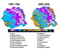Example DGVM output

Several DGVMs appeared in the middle 1990s. The first was apparently IBIS (Foley et al., 1996), VECODE (Brovkin et al., 1997), followed by several others described below:

Several DGVMs have been developed by various research groups around the world:

• LPJ^[4][5] - Germany, Sweden

• IBIS - Integrated Biosphere Simulator ^[6][7][8] - U.S.

• MC1^[9][10][11] - U.S.

• HYBRID^[12] - U.K.

• SDGVM^[13] - U.K.

• SEIB-DGVM^[14] - Japan

• TRIFFID^[15] - U.K.

• VECODE^[16] - Germany

• CLM-DVGM^[17] - U.S.

The next generation of models - earth system models (ex. CCSM^[18], ORCHIDEE^[19], JULES^[20], CTEM^[21] ) - now includes the important feedbacks from the biosphere to the atmosphere so that vegetation shifts and changes in the carbon and hydrological cycles affect the climate.

DGVMs commonly simulate a variety of plant and soil physiological processes. The processes simulated by various DGVMs are summarized in the table below. Abbreviations are: NPP, net primary production; PFT, plant functional type; SAW, soil available water; LAI, leaf area index; I, solar radiation; T, air temperature; Wr, root zone water supply; PET, potential evapotranspiration; vegc, total live vegetation carbon.

process/attribute	formulation/value	DGVMs
shortest time step	1 hour	IBIS
	2 hours	TRIFFID
	12 hours	HYBRID
	1 day	LPJ, SDGVM, SEIB-DGVM, MC1 fire submodel
	1 month	MC1 except fire submodel
	1 year	VECODE
photosynthesis	Farquhar et al. (1980)[22]	HYBRID
	Farquhar et al. (1980) Collatz et al. (1992)[23]	IBIS, LPJ, SDGVM
	Collatz et al. (1991)[24] Collatz et al. (1992)	TRIFFID
stomatal conductance	Jarvis (1976)[25] Stewart (1988)[26]	HYBRID
	Leuning (1995)[27]	IBIS, SDGVM, SEIB-DGVM
	Haxeltine & Prentice (1996)[28]	LPJ
	Cox et al. (1998)[29]	TRIFFID
production	forest NPP = f(PFT, vegc, T, SAW, P, ...) grass NPP = f(PFT, vegc, T, SAW, P, light competition, ...)	MC1
	GPP = f(I, LAI, T, Wr, PET, CO2)	LPJ
competition	for light, water, and N	MC1, HYBRID
	for light and water	LPJ, IBIS, SDGVM, SEIB-DGVM
	Lotka-Volterra in fractional cover	TRIFFID
	Climate-dependent	VECODE
establishment	All PFTs establish uniformly as small individuals	HYBRID
	Climatically favored PFTs establish uniformly, as small individuals	SEIB-DGVM
	Climatically favored PFTs establish uniformly, as small LAI increment	IBIS
	Climatically favored PFTs establish in proportion to area available, as small individuals	LPJ, SDGVM
	Minimum 'seed' fraction for all PFTs	TRIFFID
mortality	Dependent on carbon pools	HYBRID
	Deterministic baseline, wind throw, fire, extreme temperatures	IBIS
	Deterministic baseline, self-thinning, carbon balance, fire, extreme temperatures	LPJ, SEIB-DGVM
	Carbon balance, wind throw, fire, extreme temperatures	SDGVM
	Prescribed disturbance rate for each PFT	TRIFFID
	Climate-dependent, based on carbon balance	VECODE
	Self-thinning, fire, extreme temperatures, drought	MC1

Individual DGVMs usually incorporate the work of many people. Nevertheless, people who work in the field often associate with each DGVM the name of just one or just a few researchers. Listing these associations risks slighting the many hard-working but less visible contributors. To those who deserve to be on the list but are not, we apologize - and point out that anyone can edit entries in Wikipedia! Here's the list of some of the most well known DGVM modelers:

CASA and NASA-CASA - Chris Potter
CLM-DGVM -
HYBRID - Andrew Friend
IBIS - Jon Foley, Chris Kucharik, Univ. of Wisconsin
LPJ - Colin Prentice, Steven Sitch, Benjamin Smith, Wolfgang Cramer, Martin Sykes
MC1 - Jim Lenihan and Ron Neilson, U.S. Forest Service, Dominique Bachelet and Chris Daly, Oregon State University
SDGVM - Ian Woodward and Mark Lomas
TRIFFID - Peter Cox, Hadley Center
VECODE - Victor Brovkin, PIK

References:

1. ^ VEMAP Members. 1995. Vegetation/ecosystem modeling and analysis project: comparing biogeography and biogeochemistry models in a continental-scale study of terrestrial ecosystem responses to climate change and CO2 doubling. Global Biogeochemical Cycles. 9(4):407-437
2. ^ Cramer, W., A. Bondeau, F.I. Woodward, I.C. Prentice, R. Betts, V. Brovkin, P.M. Cox, V. Fischer, J.A. Foley, A.D. Friend, C. Kucharik, M.R. Lomas, N. Ramankutty, S. Sitch, B. Smith, A. White, and C. Young-Molling. 2001. Global response of terrestrial ecosystem structure and function to CO2 and climate change: results from six dynamic global vegetation models. Global Change Biology 7:357-373
3. ^ http://www.cgd.ucar.edu/vemap/
4. ^ Sitch S, Smith B, Prentice IC, Arneth A, Bondeau A, Cramer W, Kaplan JO, Levis S, Lucht W, Sykes MT, Thonicke K, Venevsky S 2003. Evaluation of ecosystem dynamics, plant geography and terrestrial carbon cycling in the LPJ Dynamic Global Vegetation Model. Global Change Biology 9, 161-185.
5. ^ http://www.pik-potsdam.de/research/cooperations/lpjweb/
6. ^ Foley, J. A., I. C. Prentice, N. Ramankutty, S. Levis, D. Pollard, S. Sitch, and A. Haxeltine. 1996. An integrated biosphere model of land surface processes, terrestrial carbon balance, and vegetation dynamics. Global Biogeochemical Cycles 10(4), 603-628.
7. ^ Kucharik, C. J., J. A. Foley, C. Delire, V. A. Fisher, M. T. Coe, J. D. Lenters, C. Young-Molling, N. Ramankutty, J. M. Norman, and S. T. Gower. 2000. Testing the performance of a Dynamic Global Ecosystem Model: Water balance, carbon balance, and vegetation structure. Global Biogeochemical Cycles 14(3), 795-825.
8. ^ Foley, J. A., C. J. Kucharik, and D. Polzin. 2005. Integrated Biosphere Simulator Model (IBIS), Version 2.5. Model product. Available on-line [1] from Oak Ridge National Laboratory Distributed Active Archive Center, Oak Ridge, Tennessee, U.S.A. doi:10.3334/ORNLDAAC/808.
9. ^ Bachelet D, Lenihan JM, Daly C, Neilson RP, Ojima DS, Parton WJ (2001). MC1: a dynamic vegetation model for estimating the distribution of vegetation and associated carbon, nutrients, and water -- technical documentation. Version 1.0. General Technical Report PNW-GTR-508. Portland, OR: U.S. Department of Agriculture, Forest Service, Pacific Northwest Research Station.
10. ^ Daly, C., D. Bachelet, J.M. Lenihan, R.P. Neilson, W. Parton, and D. Ojima, Dynamic simulation of tree-grass interactions for global change studies, Ecological Applications, 10, 449-469, 2000.
11. ^ MC1 website
12. ^ Friend AD, Stevens AK, Knox RG, Cannell MGR (1995) A process-based terrestrial biosphere model of ecosystem dynamics (Hybrid v3.0). Ecological Modelling, 95, 249-287.
13. ^ Woodward FI, Lomas MR, Betts RA (1998) Vegetation-climate feedbacks in a greenhouse world. Philos. Trans. R. soc. London, Ser. B, 353, 29-38
14. ^ http://seib-dgvm.com/
15. ^ http://www.metoffice.gov.uk/research/hadleycentre/models/carbon_cycle/models_terrest.html
16. ^ Brovkin V, Ganopolski A, Svirezhev Y (1997) A continuous climate-vegetation classification for use in climate-biosphere studies. Ecological Modelling, 101, 251-261.
17. ^ Levis SG, Bonan B, Vertenstein M, Oleson KW (2004) The Community Land Model's Dynamic Global Vegetation Model (CLM-DGVM): Technical Description and User's Guide, NCAR Tech. Note TN-459+IA, 50 pp, National Center for Atmospheric Research, Boulder, Colorado.
18. ^ http://www.ccsm.ucar.edu/
19. ^ http://orchidee.ipsl.jussieu.fr/
20. ^ http://www.jchmr.org/jules
21. ^ http://www.cccma.bc.ec.gc.ca/ctem/
22. ^ Farquhar GD, von Caemmerer S, Berry JA (1980) A biochemical model of photosynthetic CO₂ assimilation in leaves of C₃ species. Planta, 149, 78-90.
23. ^ Collatz GJ, Ribas-Carbo M, Berry JA (1992) A coupled photosynthesis - stomatal conductance model for leaves of C4 plants. Australian Journal of Plant Physiology, 19, 519-538.
24. ^ Collatz GJ, Ball JT, Grivet C, Berry JA (1991) Physiological and environmental regulation of stomatal conductance, photosynthesis and transpiration: a model that includes a laminar boundary layer. Agricultural and Forest Meteorology, 54, 107-136.
25. ^ Jarvis P (1976) The interpretation of the variations in leaf water potential and stomatal conductance found in canopies in the field. Philosophical Transactions of the Royal Society of London Series B, 273, 593-610.
26. ^ Stewart JB (1988) Modelling surface conductance of pine forest. Agricultural and Forest Meteorology, 43, 19-35.
27. ^ Leuning R (1995) A critical appraisal of a combined stomatal-photosynthesis model for C₃ plants. Plant, Cell and Environment, 18 (4), 339-355.
28. ^ Haxeltine A, Prentice IC (1996) A general model for the light-use efficiency of primary production. Functional Ecology, 10 (5), 551-561.
29. ^ Cox PM, Huntingford C, Harding RJ (1998) A canopy conductance and photosynthesis model for use in a GCM land surface scheme. Journal of Hydrology, 212-213, 79-94.