Cramer's rule

In linear algebra, Cramer's rule is a theorem, which gives an expression for the solution of a system of linear equations with as many equations as unknowns, valid in those cases where there is a unique solution. The solution is expressed in terms of the determinants of the (square) coefficient matrix and of matrices obtained from it by replacing one column by the vector of right hand sides of the equations. It is named after Gabriel Cramer (1704–1752), who published the rule in his 1750 Introduction à l'analyse des lignes courbes algébriques (Introduction to the analysis of algebraic curves), although Colin Maclaurin also published the method in his 1748 Treatise of Algebra (and probably knew of the method as early as 1729).^[1][2]

General case

Consider a system of n linear equations for n unknowns, represented in matrix multiplication form as follows:

$Ax = b\,$

$(1)\,$

where the n by n matrix A is has a nonzero determinant, and the vector $x = (x_1, \ldots, x_n)^\top$ is the column vector of the variables.

Then the theorem states that in this case the system has a unique solution, whose individual values for the unknowns are given by:

$x_i = \frac{\det(A_i)}{\det(A)} \qquad i = 1, \ldots, n \,$

where A_i is the matrix formed by replacing the ith column of A by the column vector b.

The rule holds for systems of equations with coefficients and unknowns in any field, not just in the real numbers. It has recently been shown that Cramer's rule can be implemented in O(n³) time,^[3] which is comparable to more common methods of solving systems of linear equations, such as Gaussian elimination.

Proof

The proof for Cramer's rule is very simple; in fact, it uses just two properties of determinants: linearity with respect to any given column (taking for that column a linear combination of column vectors produces as determinant the corresponding linear combination of their determinants), and the fact that the determinant is zero whenever two columns are equal (the determinant is alternating in the columns).

Fix the index j of a column. Linearity means that if we consider only column j as variable (fixing the others arbitrarily), the resulting function Rⁿ → R (assuming matrix entries are in R) can be given by a matrix, with one row and n columns. In fact this is precisely what Laplace expansion does, writing det(A) = C₁a_1,j + … + C_na_n,j for certain coefficients C₁,…,C_n that depend on the columns of A other than column j (the precise expression for these cofactors is not important here). The value det(A) is then the result of applying the one-line matrix L_(j) = (C₁ C₂ … C_n) to column j of A. If L_(j) is applied to any other column k of A, then the result is the determinant of the matrix obtained from A by replacing column j by a copy of column k, which is 0 (the case of two equal columns).

Now consider a system of n linear equations in n unknowns $x_1, x_2,\ldots,x_n$, whose coefficient matrix is A, with det(A) assumed to be nonzero:

$\begin{matrix}a_{11}x_1+a_{12}x_2+\cdots+a_{1n}x_n&=&b_1\\a_{21}x_1+a_{22}x_2+\cdots+a_{2n}x_n&=&b_2\\\vdots&\vdots&\vdots\\a_{n1}x_1+a_{n2}x_2+\cdots+a_{nn}x_n&=&b_n\end{matrix}$

If one combines these equations by taking C₁ times the first equation, plus C₂ times the second, and so forth until C_n times the last, then the coefficient of x_j will become C₁a_1,j + … + C_na_n,j = det(A), while the coefficients of all other unknowns become 0; the left hand side becomes simply det(A)x_j. The right hand side is C₁b₁ + … + C_nb_n, which is L_(j) applied to the column vector b of the right hand sides b_i. In fact what has been done here is multiply the matrix equation A ⋅ x = b on the left by L_(j). Dividing by the nonzero number det(A) one finds the following equation, necessary to satisfy the system:

$x_j=\frac{L_{(j)}\cdot\mathbf{b}}{\det(A)}.$

But by construction the numerator is determinant of the matrix obtained from A by replacing column j by b, so we get the expression of Cramers rule as necessary condition for a solution. The same procedure can be repeated for other values of j to find values for the other unknowns.

The only point that remains to prove is that these values for the unknowns, the only possible ones, to indeed together form a solution. But if the matrix A is invertible with inverse A⁻¹, then x = A⁻¹ ⋅ b will be a solution, thus showing its existence. To see that A is invertible when det(A) is nonzero, consider the n by n matrix M obtained by stacking the one-line matrices L_(j) on top of each other for j = 1, 2, …, n (this gives the adjugate matrix for A). It was shown that L_(j) ⋅ A = (0 … 0 det(A) 0 … 0) where det(A) appears at the position j; from this it follows that M ⋅ A = det(A)I_n. Therefore

$\frac1{\det(A)}M=A^{-1},$

completing the proof.

Finding inverse matrix

Main article: Invertible matrix#Methods of matrix inversion

Let A be an n×n matrix. Then

$\mathrm{Adj}(A)A = \mathrm{det}(A)I\,$

where Adj(A) denotes the adjugate matrix of A, det(A) is the determinant, and I is the identity matrix. If det(A) is invertible in R, then the inverse matrix of A is

$A^{-1} = \frac{1}{\operatorname{det}(A)} \operatorname{Adj}(A).$

If R is a field (such as the field of real numbers), then this gives a formula for the inverse of A, provided det(A) ≠ 0. In fact, this formula will work whenever R is a commutative ring, provided that det(A) is a unit. If det(A) is not a unit, then A is not invertible.

Applications

Explicit formulas for small systems

Consider the linear system $\left\{\begin{matrix}ax+by&={\color{red}e}\\ cx + dy&= {\color{red}f}\end{matrix}\right.\$ which in matrix format is $\begin{bmatrix} a & b \\ c & d \end{bmatrix}\begin{bmatrix} x \\ y \end{bmatrix}=\begin{bmatrix} {\color{red}e} \\ {\color{red}f} \end{bmatrix}.$ Then, x and y can be found with Cramer's rule as

$x = \begin{vmatrix} \color{red}{e} & b \\ \color{red}{f} & d \end{vmatrix}/\begin{vmatrix} a & b \\ c & d \end{vmatrix} = { {\color{red}e}d - b{\color{red}f} \over ad - bc}$ and

$y = \begin{vmatrix} a & \color{red}{e} \\ c & \color{red}{f} \end{vmatrix}/\begin{vmatrix} a & b \\ c & d \end{vmatrix} = { a{\color{red}f} - {\color{red}e}c \over ad - bc}.$

The rules for 3×3 are similar. Given $\left\{\begin{matrix}ax + by + cz&= {\color{red}j}\\dx + ey + fz&= {\color{red}k}\\gx + hy + iz&= {\color{red}l}\end{matrix}\right.$ which in matrix format is

$\begin{bmatrix} a & b & c \\ d & e & f \\ g & h & i \end{bmatrix}\begin{bmatrix} x \\ y \\ z \end{bmatrix}=\begin{bmatrix} {\color{red}j} \\ {\color{red}k} \\ {\color{red}l} \end{bmatrix}$ the values of x, y and z can be found as follows:

$x = \frac { \begin{vmatrix} {\color{red}j} & b & c \\ {\color{red}k} & e & f \\ {\color{red}l} & h & i \end{vmatrix} } { \begin{vmatrix} a & b & c \\ d & e & f \\ g & h & i \end{vmatrix} }, \quad y = \frac { \begin{vmatrix} a & {\color{red}j} & c \\ d & {\color{red}k} & f \\ g & {\color{red}l} & i \end{vmatrix} } { \begin{vmatrix} a & b & c \\ d & e & f \\ g & h & i \end{vmatrix} },\text{ and }z = \frac { \begin{vmatrix} a & b & {\color{red}j} \\ d & e & {\color{red}k} \\ g & h & {\color{red}l} \end{vmatrix} } { \begin{vmatrix} a & b & c \\ d & e & f \\ g & h & i \end{vmatrix} }.$

Differential geometry

Cramer's rule is also extremely useful for solving problems in differential geometry. Consider the two equations $F(x, y, u, v) = 0\,$ and $G(x, y, u, v) = 0\,$. When u and v are independent variables, we can define $x = X(u, v)\,$ and $y = Y(u, v).\,$

Finding an equation for $\dfrac{\partial x}{\partial u}$ is a trivial application of Cramer's rule.

First, calculate the first derivatives of F, G, x, and y:

$dF = \frac{\partial F}{\partial x} dx + \frac{\partial F}{\partial y} dy +\frac{\partial F}{\partial u} du +\frac{\partial F}{\partial v} dv = 0$

$dG = \frac{\partial G}{\partial x} dx + \frac{\partial G}{\partial y} dy +\frac{\partial G}{\partial u} du +\frac{\partial G}{\partial v} dv = 0$

$dx = \frac{\partial X}{\partial u} du + \frac{\partial X}{\partial v} dv$

$dy = \frac{\partial Y}{\partial u} du + \frac{\partial Y}{\partial v} dv.$

Substituting dx, dy into dF and dG, we have:

$dF = \left(\frac{\partial F}{\partial x} \frac{\partial x}{\partial u} +\frac{\partial F}{\partial y} \frac{\partial y}{\partial u} +\frac{\partial F}{\partial u} \right) du + \left(\frac{\partial F}{\partial x} \frac{\partial x}{\partial v} +\frac{\partial F}{\partial y} \frac{\partial y}{\partial v} +\frac{\partial F}{\partial v} \right) dv = 0$

$dG = \left(\frac{\partial G}{\partial x} \frac{\partial x}{\partial u} +\frac{\partial G}{\partial y} \frac{\partial y}{\partial u} +\frac{\partial G}{\partial u} \right) du + \left(\frac{\partial G}{\partial x} \frac{\partial x}{\partial v} +\frac{\partial G}{\partial y} \frac{\partial y}{\partial v} +\frac{\partial G}{\partial v} \right) dv = 0.$

Since u, v are both independent, the coefficients of du, dv must be zero. So we can write out equations for the coefficients:

$\frac{\partial F}{\partial x} \frac{\partial x}{\partial u} +\frac{\partial F}{\partial y} \frac{\partial y}{\partial u} = -\frac{\partial F}{\partial u}$

$\frac{\partial G}{\partial x} \frac{\partial x}{\partial u} +\frac{\partial G}{\partial y} \frac{\partial y}{\partial u} = -\frac{\partial G}{\partial u}$

$\frac{\partial F}{\partial x} \frac{\partial x}{\partial v} +\frac{\partial F}{\partial y} \frac{\partial y}{\partial v} = -\frac{\partial F}{\partial v}$

$\frac{\partial G}{\partial x} \frac{\partial x}{\partial v} +\frac{\partial G}{\partial y} \frac{\partial y}{\partial v} = -\frac{\partial G}{\partial v}.$

Now, by Cramer's rule, we see that:

$\frac{\partial x}{\partial u} = \frac{\begin{vmatrix} -\frac{\partial F}{\partial u} & \frac{\partial F}{\partial y} \\ -\frac{\partial G}{\partial u} & \frac{\partial G}{\partial y}\end{vmatrix}}{\begin{vmatrix}\frac{\partial F}{\partial x} & \frac{\partial F}{\partial y} \\ \frac{\partial G}{\partial x} & \frac{\partial G}{\partial y}\end{vmatrix}}.$

This is now a formula in terms of two Jacobians:

$\frac{\partial x}{\partial u} = - \frac{\left(\frac{\partial\left(F, G\right)}{\partial\left(u, y\right)}\right)}{\left(\frac{\partial\left(F, G\right)}{\partial\left(x, y\right)}\right)}.$

Similar formulae can be derived for $\frac{\partial x}{\partial v}$, $\frac{\partial y}{\partial u}$, $\frac{\partial y}{\partial v}.$

Integer programming

Cramer's rule can be used to prove that an integer programming problem whose constraint matrix is totally unimodular and whose right-hand side is integer, has integer basic solutions. This makes the integer program substantially easier to solve.

Ordinary differential equations

Cramer's rule is used to derive the general solution to an inhomogeneous linear differential equation by the method of variation of parameters.

Geometric interpretation

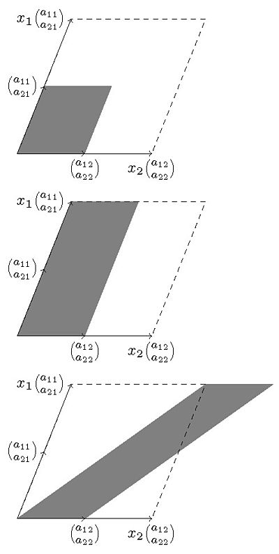Geometric interpretation of Cramer's rule. The areas of the second and third shaded parallelograms are the same and the second is x₁ times the first. From this equality Cramer's rule follows.

Cramer's rule has a geometric interpretation that can be considered also a proof or simply giving insight about its geometric nature. These geometric arguments work in general and not only in the case of two equations with two unknowns presented here.

Given the system of equations

$\begin{matrix}a_{11}x_1+a_{12}x_2&=b_1\\a_{21}x_1+a_{22}x_2&=b_2\end{matrix}$

it can be considered as an equation between vectors

$x_1\binom{a_{11}}{a_{21}}+x_2\binom{a_{12}}{a_{22}}=\binom{b_1}{b_2}.$

The area of the parallelogram determined by $\binom{a_{11}}{a_{21}}$ and $\binom{a_{12}}{a_{22}}$ is given by the determinant of the system of equations:

$\left|\begin{matrix}a_{11}&a_{12}\\a_{21}&a_{22}\end{matrix}\right|.$

In general, when there are more variables and equations, the determinant of n vectors of length n will give the volume of the parallelepiped determined by those vectors in the n-th dimensional Euclidean space.

Therefore the area of the parallelogram determined by $x_1\binom{a_{11}}{a_{21}}$ and $\binom{a_{12}}{a_{22}}$ has to be x₁ times the area of the first one since one of the sides has been multiplied by this factor. Now, this last parallelogram, by Cavalieri's principle, has the same area as the parallelogram determined by $\binom{b_1}{b_2}=x_1\binom{a_{11}}{a_{21}}+x_2\binom{a_{12}}{a_{22}}$ and $\binom{a_{12}}{a_{22}}$.

Equating the areas of this last and the second parallelogram gives the equation

$\left|\begin{matrix}b_1&a_{12}\\b_2&a_{22}\end{matrix}\right|=\left|\begin{matrix}a_{11}x_1&a_{12}\\a_{21}x_1&a_{22}\end{matrix}\right|=x_1\left|\begin{matrix}a_{11}&a_{12}\\a_{21}&a_{22}\end{matrix}\right|$

from which Cramer's rule follows.

Incompatible and indeterminate cases

A system of equations is said to be incompatible when there are no solutions and it is called indeterminate when there is more than one solution. For linear equations, an indeterminate system will have infinitely many solutions (if it is over an infinite field), since the solutions can be expressed in terms of one or more parameters that can take arbitrary values.

Cramer's rule applies to the case where the coefficient determinant is nonzero. In the contrary case the system is either incompatible or indeterminate, based on the values of the determinants only for 2x2 systems.

For 3x3 or higher systems, the only thing one can say when the coefficient determinant equals zero is: if any of the "numerator" determinants are nonzero, then the system must be incompatible. However, the converse is false: having all determinants zero does not imply that the system is indeterminate. A simple example where all determinants vanish but the system is still incompatible is the 3x3 system x+y+z=1, x+y+z=2, x+y+z=3.

See also

• Matrix

Notes

1. ^ Carl B. Boyer, A History of Mathematics, 2nd edition (Wiley, 1968), p. 431.
2. ^ Victor Katz, A History of Mathematics, Brief edition (Pearson Education, 2004), pp. 378–379.
3. ^ Ken Habgood, Itamar Arel, A condensation-based application of Cramerʼs rule for solving large-scale linear systems, Journal of Discrete Algorithms, ISSN 1570-8667, 10.1016/j.jda.2011.06.007.

External links

• Proof of Cramer's Rule
• WebApp descriptively solving systems of linear equations with Cramer's Rule
• Cramer's Rule Solver
• Online Calculator of System of linear equations