- Metropolis–Hastings algorithm
-

In mathematics and physics, the Metropolis–Hastings algorithm is a Markov chain Monte Carlo method for obtaining a sequence of random samples from a probability distribution for which direct sampling is difficult. This sequence can be used to approximate the distribution (i.e., to generate a histogram), or to compute an integral (such as an expected value).
Contents
History
The algorithm was named after Nicholas Metropolis, who was an author along with Arianna W. Rosenbluth, Marshall N. Rosenbluth, Augusta H. Teller, and Edward Teller of the 1953 paper Equation of State Calculations by Fast Computing Machines which first proposed the algorithm for the specific case of the Boltzmann distribution;[1] and W. Keith Hastings,[2] who extended it to the more general case in 1970.[3] There is controversy over the credit for discovery of the algorithm. Edward Teller states in his memoirs that the five authors of the 1953 paper worked together for "days (and nights)".[4] M. Rosenbluth, in an oral history recorded shortly before his death [5] credits E. Teller with posing the original problem, himself with solving it, and A.W. Rosenbluth (his wife) with programming the computer. According to M. Rosenbluth, neither Metropolis nor A.H. Teller participated in any way. Rosenbluth's account of events is supported by other contemporary recollections.[6]
The Gibbs sampling algorithm is a special case of the Metropolis–Hastings algorithm which is usually faster and easier to use but is less generally applicable.
Overview
The Metropolis–Hastings algorithm can draw samples from any probability distribution
 , requiring only that a function that is proportional to the density be calculable. In Bayesian applications, the normalization factor is often extremely difficult to compute, so the ability to generate a sample without knowing this constant of proportionality is a major virtue of the algorithm.
The general idea of the algorithm is to use a Markov chain that, at sufficiently long times, generates states that obey the
distribution. To this purpose, the Markov chain must fulfill two conditions: ergodicity and condition of balance, which is generally obtained if it fulfills detailed balance (a stronger condition). The ergodicity condition ensures that at most, one asymptotic distribution exists. The detailed balance condition ensures that there exists at least one asymptotic distribution.A Markov chain generates a new state
 that depends only on the previous state
  . The algorithm uses a proposal density
  , which depends on the current state , to generate a new proposed sample
  . This proposal is "accepted" as the next value (
 ) if
) if  drawn from
  , the uniform distribution, satisfies
If the proposal is not accepted, then the current value of
 is retained:
  .
.For example, the proposal density could be a Gaussian function centered on the current state
:reading
as the probability density function for given the previous value . This proposal density would generate samples centered around the current state with variance  . The original Metropolis algorithm calls for the proposal density to be symmetric
  ; the generalization by Hastings lifts this restriction. It is also permissible for not to depend on at all, in which case the algorithm is called "Independence Chain Metropolis-Hastings" (as opposed to "Random Walk Metropolis-Hastings"). The Independence Chain M-H algorithm with a suitable proposal density function can reduce serial correlation and offer higher efficiency than the random walk version, but it requires some a priori knowledge of the distribution.
Step-by-step instructions
Suppose the most recent value sampled is
 . To follow the Metropolis–Hastings algorithm, we next draw a new proposal state
  with probability density
  , and calculate a value
where
is the likelihood ratio between the proposed sample
and the previous sample , andis the ratio of the proposal density in two directions (from
to and vice versa). This is equal to 1 if the proposal density is symmetric. Then the new state is chosen according to the following rules.The Markov chain is started from an arbitrary initial value
 and the algorithm is run for many iterations until this initial state is "forgotten". These samples, which are discarded, are known as burn-in. The remaining set of accepted values of x represent a sample from the distribution P(x).
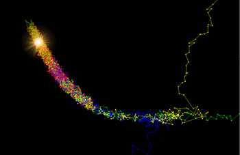 The result of three Markov chains running on the 3D Rosenbrock function using the Metropolis-Hastings algorithm. The algorithm samples from regions where the posterior probability is high and the chains begin to mix in these regions. The approximate position of the maximum has been illuminated. Note that the red points are the ones that remain after the burn-in process. The earlier ones have been discarded.
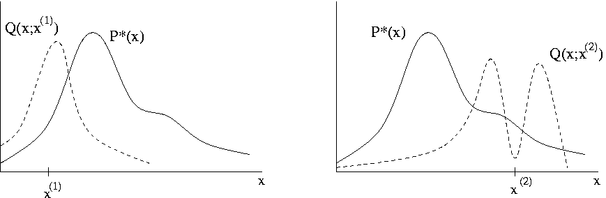
The algorithm works best if the proposal density matches the shape of the target distribution
from which direct sampling is difficult, that is  . If a Gaussian proposal density
  is used the variance parameter
  has to be tuned during the burn-in period. This is usually done by calculating the acceptance rate, which is the fraction of proposed samples that is accepted in a window of the last
  samples. The desired acceptance rate depends on the target distribution, however it has been shown theoretically that the ideal acceptance rate for a one dimensional Gaussian distribution is approx 50%, decreasing to approx 23% for an -dimensional Gaussian target distribution.[7] If is too small the chain will mix slowly (i.e., the acceptance rate will be high but successive samples will move around the space slowly and the chain will converge only slowly to ). On the other hand, if is too large the acceptance rate will be very low because the proposals are likely to land in regions of much lower probability density, so
  will be very small and again the chain will converge very slowly.
See also
- Simulated annealing
- Detailed balance
- Multiple-try Metropolis
- Metropolis light transport
- Gibbs sampling
Notes
- ^ Metropolis, N.; Rosenbluth, A.W.; Rosenbluth, M.N.; Teller, A.H.; Teller, E. (1953). "Equations of State Calculations by Fast Computing Machines". Journal of Chemical Physics 21 (6): 1087–1092. Bibcode 1953JChPh..21.1087M. doi:10.1063/1.1699114.
- ^ Rosenthal, Jeffrey (March 2004). "W.K. Hastings, Statistician and Developer of the Metropolis-Hastings Algorithm". http://probability.ca/hastings/. Retrieved 2009-06-02.
- ^ Hastings, W.K. (1970). "Monte Carlo Sampling Methods Using Markov Chains and Their Applications". Biometrika 57 (1): 97–109. doi:10.1093/biomet/57.1.97. JSTOR 2334940. Zbl 0219.65008.
- ^ Teller, Edward. "Memoirs: A Twentieth-Century Journey in Science and Politics". Perseus Publishing, 2001, p. 328
- ^ Rosenbluth, Marshall. "Oral History Transcript". American Institute of Physics
- ^ J.E. Gubernatis (2005). "Marshall Rosenbluth and the Metropolis Algorithm". Physics of Plasmas 12: 057303. Bibcode 2005PhPl...12e7303G. doi:10.1063/1.1887186.
- ^ Roberts, G.O.; Gelman, A.; Gilks, W.R. (1997). "Weak convergence and optimal scaling of random walk Metropolis algorithms". Ann. Appl. Probab. 7 (1): 110–120. doi:10.1214/aoap/1034625254.
References
- Bernd A. Berg. Markov Chain Monte Carlo Simulations and Their Statistical Analysis. Singapore, World Scientific 2004.
- Siddhartha Chib and Edward Greenberg: "Understanding the Metropolis–Hastings Algorithm". American Statistician, 49(4), 327–335, 1995
- Bolstad, William M. (2010) Understanding Computational Bayesian Statistics, John Wiley ISBN 0-470-04609-8
External links
Categories:- Monte Carlo methods
- Markov chain Monte Carlo
- Statistical algorithms


Wikimedia Foundation. 2010.