Polyharmonic spline

In mathematics, polyharmonic splines are used for
function approximation and data interpolation.They are very useful for interpolation of scattered datain many dimensions.

Polyharmonic splines are a special case of radial basis functions andare defined as a linear combination of non-linear basis functions$phi(.)$ that depend only on distancestogether with a low order polynomial (for notational simplicity, in thesequel only linear polynomials are treated):

where

---

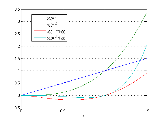
thumb|350px|right|Polyharmonic basis functions
* $mathbf\{x\}\; =\; [x\_1,\; x\_2,\; cdots,\; x\_\{nx\}]\; ^T$ is a real-valued vector of nx independent variables,
* $mathbf\{c\}\_i\; =\; [c\_\{1,i\},\; c\_\{2,i\},\; cdots,\; c\_\{nx,i\}]\; ^T$ are N vectors of the same size as $mathbf\{x\}$ (often called center).
* $mathbf\{w\}\; =\; [w\_1,\; w\_2,\; cdots,\; w\_N]\; ^T$ are the N weights of the basis functions.
* $mathbf\{v\}\; =\; [v\_1,\; v\_2,\; cdots,\; v\_\{nx+1\}]\; ^T$ are the nx+1 weights of the polynomial.
* The linear polynomial with the weighting factors $mathbf\{v\}$ improves the interpolation close to the "boundary" and expecially the extrapolation "outside" of the centers $mathbf\{c\}\_i$. If this is not desired, this term can also be removed (see also figure) below.

The basis functions of polyharmonic splines are radial basis functions of the form:

Other values of exponent k are not useful (such as $phi(r)\; =\; r^2$),because a solution of the interpolation problem might nolonger exist. To avoid problems at r=0 (since ln(0) = -∞), the polyharmonic splines with the natural logarithm might be implemented as:

The weights $w\_i$ and $v\_j$ are determined such that the functionpasses through $N$ given points$(mathbf\{c\}\_i,\; y\_i)$ (i=1,2,...,N) and fulfill the $nx+1$ orthogonality conditions:

$0\; =\; sum\_\{i=1\}^N\; w\_i,\; ;;\; 0\; =\; sum\_\{i=1\}^N\; w\_i\; ,\; c\_\{j,i\}\; ;;;\; (j=1,2,...,nx)$

In order to compute the weights, a symmetric, linear system of equations has to besolved:

where

Under very mild conditions (essentially, that at least nx+1 pointsare not in a subspace; e.g. for nx=2 that at least 3 points are noton a straight line), the system matrix of the linear system of equationsis positiv definite and therefore a unique solution of the equation systemexists.

Once the weights are determined, interpolation requires to just evaluate thetop most formula for the provided $mathbf\{x\}$.

The main advantage of polyharmonic spline interpolation isthat usually very good interpolationresults are obtained for scattered data without performing any "tuning", so automatic interpolation is feasible. This is not the case forother radial basis functions. For example, the Gaussian function($e^\{-kcdot\; r^2\}$) needs to be tuned, so that k is selectedaccording to the underlying grid of the independent variables. If this gridis non-uniform, a proper selection of k is difficult or impossible, in orderto achieve a good interpolation result.

The main disadvantages are

* In order to determine the weights, a linear system of equations has to be solved, which is non-sparse. The solution of a non-sparse linear system becomes no longer practical if the dimension n is larger as about 1000 (since the storage requirements are O(n²) and the number of operations to solve the linear system is O(n³). For example n=10000 requires about 100 Mbyte of storage and 1000 Gflops of operations).

* In order to perform the interpolation of M data points, operations in the order of O(M*N) are needed. In many applications, like image processing, M is much larger as N, and if both numbers are large, this is no longer practical.

Recently, methods have been developed to overcome the mentioned difficulties,see, e.g., [http://imajna.oxfordjournals.org/cgi/content/short/27/3/427 (Beatson et.al. 2006)]

---

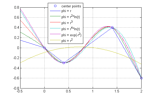
frame|none|Interpolation with different polyharmonic splines that shall pass the 4 predefined points marked by a circle (the interpolation with phi = r">² is not useful, since the linear equation system of the interpolation problem has no solution; it is solved in a least squaressense, but then does not pass the centers)

The figure shows the interpolation through four points (marked by "circles") using different types of polyharmonic splines. The "curvature" of the interpolated curves grows with the order of the spline and the extrapolation at the left boundary (x < 0) is reasonable. The figure also includes the radial basis functions phi = exp(-r²) which gives a good interpolation as well. Finally, the figure includes alsothe non-polyharmonic spline phi = r² to demonstrate, that thisradial basis function is not able to pass through the predefined points(the linear equation has no solution and is solved in a least squares sense).

The figure shows the same interpolation as in the first figure, with the only exception that the points to be interpolated are scaled by a factor of 100 (and the case phi = r² is no longer included). Since phi = (scale*r)^k =(scale^k)*r^k, the factor (scale^k) can be extracted from matrix A of the linear equation system and therefore the solution is not influenced by the scaling. This is different for the logarithmic form of the spline, although the scaling has not much influence. This analysis is reflected in the figure, where the interpolation shows not much differences. Note, for other radial basis functions, such as phi = exp(-k*r²) with k=1, the interpolation is no longer reasonable and it would be necessary to adapt k.

The figure shows the same interpolation as in the first figure, withthe only exception that the polynomial term of the function is nottaken into account (and the case phi = r² is no longer included). As can be seen from the figure, the extrapolation for x < 0 is no longer as "natural" as in the first figure for some of the basis functions. This indicates, that the polynomial term is useful if extrapolation occurs.

ee also

*Radial basis function
*Subdivision surface (emerging alternative to spline-based surfaces)
*Spline
*Thin plate spline (a special case of a polyharmonic spline)

References

* Beatson R.K., Powell M.J.D., and Tan A.M. (2006): [http://imajna.oxfordjournals.org/cgi/content/short/27/3/427 Fast evaluation of polyharmonic splines in three dimensions] .
* Fasshauer G.F. (2007): [http://books.google.com/books?id=gtqBdMEqryEC Meshfree Approximation Methods with MATLAB] . World Scientific Publishing Company, ISPN-10: 9812706348
* Iske A. (2004): [http://www.springeronline.com/sgw/cda/frontpage/0,10735,5-10042-22-22344683-0,00.html Multiresolution Methods in Scattered Data Modelling] , Lecture Notes in Computational Science and Engineering, Vol. 37, ISBN 3-540-20479-2, Springer-Verlag, Heidelberg.
* Scott A. Sarra (2006): "Integrated Multiquadric Radial Basis Function Approximation Methods", "Computers and Mathematics with Applications", vol. 51, no. 8, pp. 1283–1296.