Collision response

In the context of classical mechanics simulations and physics engines employed within video games, collision response deals with models and algorithms for simulating the changes in the motion of two solid bodies following collision and other forms of contact.

Rigid Body Contact

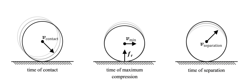
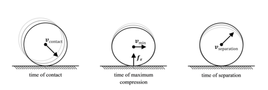The compression and expansion phases of a collision between two solid bodies

Two rigid bodies in unconstrained motion, potentially under the action of forces, may be modelled by solving their equations of motion using numerical integration techniques. On collision, the kinetic properties of two such bodies seem to undergo an instantaneous change, typically resulting in the bodies rebounding away from each other, sliding, or settling into relative static contact, depending on the elasticity of the materials and the configuration of the collision.

Contact Forces

The origin of the rebound phenomenon, or reaction, may be traced to the behaviour of real bodies that, unlike their perfectly rigid idealised counterparts, do undergo minor compression on collision, followed by expansion, prior to separation. The compression phase converts the kinetic energy of the bodies into potential energy and to an extent, heat. The expansion phase converts the potential energy back to kinetic energy.

During the compression and expansion phases of two colliding bodies, each body generates reactive forces on the other at the points of contact, such that the sum reaction forces of one body are equal in magnitude but opposite in direction to the forces of the other, as per the Newtonian principle of action and reaction. If the effects of friction are ignored, a collision is seen as affecting only the component of the velocities that are directed along the contact normal and as leaving the tangential components unaffected

Reaction

The degree of relative kinetic energy retained after a collision, termed the restitution, is dependent on the elasticity of the bodies‟ materials. The coefficient of restitution between two given materials is modeled as the ratio $e \in [0..1]$ of the relative post-collision speed of a point of contact along the contact normal, with respect to the relative pre-collision speed of the same point along the same normal. These coefficients are typically determined empirically for different material pairs, such as wood against concrete or rubber against wood. Values for e close to zero indicate inelastic collisons such as a piece of soft clay hitting the floor, whereas values close to one represent highly elastic collisions, such as a rubber ball bouncing off a wall. The kinetic energy loss is relative to one body with respect to the other. Thus the total momentum of both bodies with respect to some common reference is unchanged after the collision, in line with the principle of conservation of momentum.

Friction

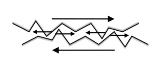Friction due to surface microstructure imperfections

Another important contact phenomenon is surface-to-surface friction, a force that impedes the relative motion of two surfaces in contact, or that of a body in a fluid. In this section we discuss surface-to-surface friction of two bodies in relative static contact or sliding contact. In the real world, friction is due to the imperfect microstructure of surfaces whose protrusions interlock into each other, generating reactive forces tangential to the surfaces.

To overcome the friction between two bodies in static contact, the surfaces must somehow lift away from each other. Once in motion, the degree of surface affinity is reduced and hence bodies in sliding motion tend to offer lesser resistance to motion. These two categories of friction are respectively termed static friction and dynamic friction.

Impulse-Based Contact Model

A force $\mathbf{f}(t)\in \mathbb{R}^3$, dependent on time $t \in\mathbb{R}$, acting on a body of assumed constant mass $m \in \mathbb{R}$ for a time interval [t₀..t₁] generates a change in the body’s momentum $\mathbf{p}(t)=m\mathbf{v}(t)$, where $\mathbf{v}(t)$ is the resulting change in velocity. The change in momentum, termed an impulse and denoted by $j \in \mathbb{R}^3$ is thus computed as

$\mathbf{j}=\int_{t_0}^{t_1}\mathbf{f}dt$

For fixed impulse $\mathbf{j}$, the equation suggests that $t_1 \rightarrow t_0 \Rightarrow \left | \mathbf{f} \right | \rightarrow \infty$, that is, a smaller time interval must be compensated by a stronger reaction force to achieve the same impulse. When modelling a collision between idealized rigid bodies, it is impractical to simulate the compression and expansion phases of the body geometry over the collision time interval. However, by assuming that a suitable force $\mathbf{f}$ can be found such that the limit

$\lim_{t_1 \rightarrow t_0} \int_{t_0}^{t_1}\mathbf{f}dt$

exists and is equal to $\mathbf{j}$, the notion of instantaneous impulses may be introduced to simulate an instantaneous change in velocity after a collision.

Impulse-Based Reaction Model

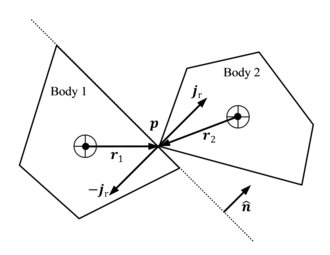The application of impulses at the point of collision

The effect of the reaction force $\mathbf{f}_r(t)\in \mathbb{R}^3$ over the interval of collision [t₀..t₁] may hence be represented by an instantaneous reaction impulse $\mathbf{j}_r(t)\in \mathbb{R}^3$, computed as

$\mathbf{j}_r=\int_{t_0}^{t_1}\mathbf{f}_r dt$

By deduction from the principle of action and reaction, if the collision impulse applied by the first body on the second body at a contact point $\mathbf{p}_r\in \mathbb{R}^3$ is $\mathbf{j}_r$, the counter impulse applied by the second body on the first is $-\mathbf{j}_r$. The decomposition $\pm \mathbf{j}_r = \pm j_r \mathbf{\hat{n}}$ into the impulse magnitude $j_r \in \mathbb{R}$ and direction along the contact normal $\mathbf{\hat{n}}$ and its negation $- \mathbf{\hat{n}}$ allows for the derivation of a formula to compute the change in linear and angular velocities of the bodies resulting from the collision impulses. In the subsequent formulas, $\mathbf{\hat{n}}$ is always assumed to point away from body 1 and towards body 2 at the contact point.

Assuming the collision impulse magnitude $\mathbf{j}_r$ is given, the change in the bodies’ velocities at the point of contact is computed as follows

	$\mathbf{v'}_1 = \mathbf{v}_1 - \frac {j_r} {m_1} \mathbf{\hat{n}}$	(1a)
	$\mathbf{v'}_2 = \mathbf{v}_2 + \frac {j_r} {m_2} \mathbf{\hat{n}}$	(1b)

where, for the ith body, $\mathbf{v}_i\in \mathbb{R}^3$ is the pre-collision velocity of the point of contact, $\mathbf{v'}_i \in \mathbb{R}^3$ is its post-collision velocity and $m_i\in \mathbb{R}$ is the mass.

The impulse yields a change in both the linear and angular components of the bodies' velocities. The angular components are calculated as follows:

	$\mathbf{\omega'}_1 = \mathbf{\omega}_1 - j_r \mathbf{I}_1^{-1} ( \mathbf{r}_1 \times \mathbf{\hat{n}} )$	(2a)
	$\mathbf{\omega'}_2 = \mathbf{\omega}_2 + j_r \mathbf{I}_2^{-1} ( \mathbf{r}_2 \times \mathbf{\hat{n}} )$	(2b)

where, for the ith body, ${\omega}_i\in \mathbb{R}^3$ is the angular pre-collision velocity, ${\omega'}_i\in \mathbb{R}^3$ is the angular post-collision velocity, $\mathbf{I}_i\in \mathbb{R}^{3 \times 3}$ is the inertia tensor in the world frame of reference, and $\mathbf{r}_i \in \mathbb{R}^3$ is offset of the shared contact point $\mathbf{p}$ from the centre of mass.

The velocities $v_{p1},v_{p2} \in \mathbb{R}^3$ of the bodies at the point of contact may be computed in terms of the respective linear and angular velocities, using

$\mathbf{v}_{pi}=\mathbf{v}_i+\mathbf{\omega}_i \times \mathbf{r}_i$

(3)

for i = 1,2. The coefficient of restitution e relates the pre-collision relative velocity $\mathbf{v}_r = \mathbf{v}_{p2} - \mathbf{v}_{p1}$ of the contact point to the post-collision relative velocity $\mathbf{v'}_r = \mathbf{v'}_{p2} - \mathbf{'v}_{p1}$ along the contact normal $\mathbf{\hat{n}}$ as follows

$\mathbf{v'}_r \cdot \mathbf{\hat{n}} = -e \mathbf{v}_r \cdot \mathbf{\hat{n}}$

(4)

Substituting equations (1a), (1b), (2a), (2b) and (3) into equation (4) and solving for the reaction impulse magnitude j_r yields

$j_r = \frac { -(1+e) \mathbf{v}_r \cdot \mathbf{\hat{n}} } { {m_1}^{-1} + {m_2}^{-1} + ({\mathbf{I}_1}^{-1} (\mathbf{r}_1 \times \mathbf{\hat{n}} ) \times \mathbf{r}_1 + {\mathbf{I}_2}^{-1} (\mathbf{r}_2 \times \mathbf{\hat{n}} ) \times \mathbf{r}_2) \cdot \mathbf{\hat{n}} }$

(5)

Computing Impulse-Based Reaction

Thus, the procedure for computing the post-collision linear velocities $\mathbf{v'}_i$ and angular velocities $\mathbf{\omega'}_i$ is as follows:

1. Compute the reaction impulse magnitude j_r in terms of $\mathbf{v}_r$, m₁, m₂, $\mathbf{I}_1$, $\mathbf{I}_2$, $\mathbf{r}_1$, $\mathbf{r}_2$, $\mathbf{\hat{n}}$ and e using equation (5)
2. Compute the reaction impulse vector $\mathbf{j}_r$ in terms of its magnitude j_r and contact normal $\mathbf{\hat{n}}$ using $\mathbf{j}_r = j_r \mathbf{\hat{n}}$.
3. Compute new linear velocities $\mathbf{v'}_i$ in terms of old velocities $\mathbf{v}_i$, masses m_i and reaction impulse vector $\mathbf{j}_r$ using equations (1a) and (1b)
4. Compute new angular velocities $\mathbf{\omega'}_i$ in terms of old angular velocities $\mathbf{\omega}_i$, interia tensors $\mathbf{I}_i$ and reaction impulse vector $\mathbf{j}_r$ using equations (2a) and (2b)

Impulse-Based Friction Model

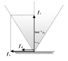Coulomb friction model - friction cone

One of the most popular models for describing friction is the Coulomb friction model. This model defines coefficients of static friction ${\mu}_s \in \mathbb{R}$ and dynamic friction ${\mu}_d \in \mathbb{R}$ such that μ_s > μ_d. These coefficients describe the two types of friction forces in terms of the reaction forces acting on the bodies. More specifically, the static and dynamic friction force magnitudes $f_s, f_d \in \mathbb{R}$ are computed in terms of the reaction force magnitude $f_r=|\mathbf{f}_r|$ as follows

	fs = μsfr	(6a)
	fd = μdfr	(6b)

The value f_s defines a maximum magnitude for the friction force required to counter the tangential component of any external sum force applied on a relatively static body, such that it remains static. Thus, if the external force is large enough, static friction is unable to fully counter this force, at which point the body gains velocity and becomes subject to dynamic friction of magnitude f_d acting against the sliding velocity.

The Coulomb friction model effectively defines a friction cone within which the tangential component of a force exerted by one body on the surface of another in static contact, is countered by an equal and opposite force such that the static configuration is maintained. Conversely, if the force falls outside the cone, static friction gives way to dynamic friction.

Given the contact normal $\mathbf{\hat{n}} \in \mathbb{R}^3$ and relative velocity $\mathbf{v}_r \in \mathbb{R}^3$ of the contact point, a tangent vector $\mathbf{\hat{t}} \in \mathbb{R}^3$, orthogonal to $\mathbf{\hat{n}}$, may be defined such that

$\mathbf{\hat{t}}=\left \{ \begin{matrix} \frac{\mathbf{v}_r - (\mathbf{v}_r \cdot \mathbf{\hat{n}})\mathbf{\hat{n}}} {|\mathbf{v}_r - (\mathbf{v}_r \cdot \mathbf{\hat{n}})\mathbf{\hat{n}}|} & \mathbf{v}_r \cdot \mathbf{\hat{n}} \neq 0 & \\ \frac{\mathbf{f}_e - (\mathbf{f}_e \cdot \mathbf{\hat{n}})\mathbf{\hat{n}}} {|\mathbf{f}_e - (\mathbf{f}_e \cdot \mathbf{\hat{n}})\mathbf{\hat{n}}|} & \mathbf{v}_r \cdot \mathbf{\hat{n}} = 0 & \mathbf{f}_e \cdot \mathbf{\hat{n}} \neq 0 \\ \mathbf{0} & \mathbf{v}_r \cdot \mathbf{\hat{n}} = 0 & \mathbf{f}_e \cdot \mathbf{\hat{n}} = 0 \\ \end{matrix}\right.$

(7)

where $\mathbf{f}_e \in \mathbb{R}^3$ is the sum of all external forces on the body. The multi-case definition of $\mathbf{\hat{t}}$ is required for robustly computing the actual friction force $\mathbf{f}_f \in \mathbb{R}^3$ for both the general and particular states of contact. Informally, the first case computes the tangent vector along the relative velocity component perpendicular to the contact normal $\mathbf{\hat{n}}$. If this component is zero, the second case derives $\mathbf{\hat{t}}$ in terms of the tangent component of the external force $\mathbf{f}_e \in \mathbb{R}^3$. If there is no tangential velocity or external forces, than no friction is assumed, and $\mathbf{\hat{t}}$ may be set to the zero vector. Thus, $\mathbf{f}_f \in \mathbb{R}^3$ is computed as

$\mathbf{f}_f=\left \{ \begin{matrix} -(\mathbf{f}_e \cdot \mathbf{\hat{t}})\mathbf{\hat{t}} & \mathbf{v}_r \cdot \mathbf{\hat{t}} = 0 & \mathbf{f}_e \cdot \mathbf{\hat{t}} \le f_s\\ -f_d \mathbf{\hat{t}} & \text{(otherwise)} \\ \end{matrix}\right.$

(8)

Equations (6a), (6b), (7) and (8) describe the Coulomb friction model in terms of forces. By adapting the argument for instantaneous impulses, an impulse-based version of the Coulomb friction model may be derived, relating a frictional impulse $\mathbf{j}_f \in \mathbb{R}^3$, acting along the tangent $\mathbf{\hat{t}}$, to the reaction impulse $\mathbf{j}_r \in \mathbb{R}^3$. Integrating (6a) and (6b) over the collision time interval [t₀..t₁] yields

	js = μsjr	(9a)
	jd = μdjr	(9b)

where $j_r=|\mathbf{j}_r |$ is the magnitude of the reaction impulse acting along contact normal $\mathbf{\hat{n}}$. Similarly, by assuming $\mathbf{\hat{t}}$ constant throughout the time interval, the integration of (8) yields

$\mathbf{j}_f=\left \{ \begin{matrix} -(m \mathbf{v}_r \cdot \mathbf{\hat{t}})\mathbf{\hat{t}} & \mathbf{v}_r \cdot \mathbf{\hat{t}} = 0 & m \mathbf{v}_r \cdot \mathbf{\hat{t}} \le j_s\\ -j_d \mathbf{\hat{t}} & \text{(otherwise)} \\ \end{matrix}\right.$

(10)

Equations (5) and (10) define an impulse-based contact model that is ideal for impulse-based simulations. When using this model, care must be taken in the choice of μ_s and μ_d as higher values may introduce additional kinetic energy into the system.

Notes

References

• C. Vella, "Gravitas: An extensible physics engine framework using object-oriented and design pattern-driven software architecture principles," Master in Information Technology Thesis, University of Malta, Msida, 2008.