CHSH inequality

In physics, the CHSH Bell test is an application of Bell's theorem, intended to distinguish between the entanglement hypothesis of quantum mechanics and local hidden variable theories. CHSH stands for John Clauser, Michael Horne, Abner Shimony and Richard Holt, who described it in a much-cited paper published in 1969 (Clauser, 1969). They derived the CHSH inequality, which, as with John Bell's original one (Bell, 1964), applies to a statistical property of counts of "coincidences" in a Bell test experiment that follows from the assumption that there exist underlying local hidden variables. The inequality must be obeyed under local realism but can be infringed under certain conditions in quantum mechanics.

Statement of the inequality

The usual form of the CHSH inequality is:

(1)       − 2 ≤ S ≤ 2,

where

(2)       S = E(a, b) − E(a, b′) + E(a′, b) + E(a′ b′).

a and a′ are detector settings on side A, b and b′ on side B, the four combinations being tested in separate subexperiments. The terms E(a, b) etc. are the quantum correlations of the particle pairs, where the quantum correlation is defined to be the expectation value of the product of the "outcomes" of the experiment, i.e. the statistical average of A(a)·B(b), where A and B are the separate outcomes, using the coding +1 for the '+' channel and −1 for the '−' channel. Clauser et al.'s 1969 derivation was oriented towards the use of "two-channel" detectors, and indeed it is for these that it is generally used, but under their method the only possible outcomes were +1 and −1. In order to adapt it to real situations, which at the time meant the use of polarised light and single-channel polarisers, they had to interpret '−' as meaning "non-detection in the '+' channel", i.e. either '−' or nothing. They did not in the original article discuss how the two-channel inequality could be applied in real experiments with real imperfect detectors, though it was later proved (Bell, 1971) that the inequality itself was equally valid. The occurrence of zero outcomes, though, means it is no longer so obvious how the values of E are to be estimated from the experimental data.

The mathematical formalism of quantum mechanics predicts a maximum value for S of $2\sqrt 2$, which is greater than 2, and CHSH violations are therefore predicted by the theory of quantum mechanics.

Note that in all actual Bell test experiments it is assumed that the source stays essentially constant, being characterised at any given instant by a state ("hidden variable") λ that has a constant distribution ρ(λ) and is unaffected by the choice of detector setting.

A typical CHSH experiment

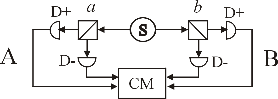
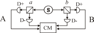Schematic of a "two-channel" Bell test
The source S produces pairs of photons, sent in opposite directions. Each photon encounters a two-channel polariser whose orientation can be set by the experimenter. Emerging signals from each channel are detected and coincidences counted by the coincidence monitor CM.

In practice most actual experiments have used light rather than the electrons that Bell originally had in mind. The property of interest is, in the best known experiments (Aspect, 1981-2), the polarisation direction, though other properties can be used. The diagram shows a typical optical experiment. Coincidences (simultaneous detections) are recorded, the results being categorised as '++', '+−', '−+' or '−−' and corresponding counts accumulated.

Four separate subexperiments are conducted, corresponding to the four terms E(a, b) in the test statistic S ((2) above). The settings a, a′, b and b′ are generally in practice chosen to be 0, 45°, 22.5° and 67.5° respectively — the "Bell test angles" — these being the ones for which the QM formula gives the greatest violation of the inequality.

For each selected value of a and b, the numbers of coincidences in each category (N₊₊, N_--, N_+- and N_-+) are recorded. The experimental estimate for E(a, b) is then calculated as:

$(3) E = \frac {N_{++} + N_{--} - N_{+-} - N_{-+}} {N_{++} + N_{--} + N_{+-} + N_{-+}}$

Once all the E’s have been estimated, an experimental estimate of S (expression (2)) can be found. If it is numerically greater than 2 it has infringed the CHSH inequality and the experiment is declared to have supported the QM (Quantum Mechanics) prediction and ruled out all local hidden variable theories.

The CHSH paper lists many preconditions (or "reasonable and/or presumable assumptions") to derive the simplified theorem and formula. For example, for the method to be valid, it has to be assumed that the detected pairs are a fair sample of those emitted. In actual experiments, detectors are never 100% efficient, so that only a sample of the emitted pairs are detected. A subtle, related requirement is that the hidden variables do not influence or determine detection probability in a way that would lead to different samples at each arm of the experiment.

Derivation of the CHSH inequality

The original 1969 derivation will not be given here since it is not easy to follow and involves the assumption that the outcomes are all +1 or −1, never zero. Bell's 1971 derivation is more general. He effectively assumes the "Objective Local Theory" later used by Clauser and Horne (Clauser, 1974). It is assumed that any hidden variables associated with the detectors themselves are independent on the two sides and can be averaged out from the start. Another derivation of interest is given in Clauser and Horne's 1974 paper, in which they start from the CH74 inequality.

It would appear from both these later derivations that the only assumptions really needed for the inequality itself (as opposed to the method of estimation of the test statistic) are that the distribution of the possible states of the source remains constant and the detectors on the two sides act independently.

Bell's 1971 derivation

The following is based on page 37 of Bell's Speakable and Unspeakable (Bell, 1971), the main change being to use the symbol ‘E’ instead of ‘P’ for the expected value of the quantum correlation. This avoids any implication that the quantum correlation is itself a probability.

We start with the standard assumption of independence of the two sides, enabling us to obtain the joint probabilities of pairs of outcomes by multiplying the separate probabilities, for any selected value of the "hidden variable" λ. λ is assumed to be drawn from a fixed distribution of possible states of the source, the probability of the source being in the state λ for any particular trial being given by the density function ρ(λ), the integral of which over the complete hidden variable space is 1. We thus assume we can write:

$E(a, b) = \int \underline {A}(a, \lambda)\underline {B}(b, \lambda)\rho(\lambda)d\lambda \qquad (4)$

where A and B are the average values of the outcomes. Since the possible values of A and B are −1, 0 and +1, it follows that:

$|\underline {A}| \leq 1, |\underline {B}| \leq 1 \qquad (5)$

Then, if a, a′, b and b′ are alternative settings for the detectors,

$E(a, b) - E(a, b^\prime) = \int [\underline {A}(a, \lambda)\underline {B}(b, \lambda) - \underline {A}(a, \lambda)\underline {B}(b^\prime, \lambda)]\rho(\lambda)d\lambda$ $= \int \underline {A}(a, \lambda)\underline {B}(b, \lambda)[1 \pm \underline {A}(a^\prime, \lambda)\underline {B}(b^\prime, \lambda)]\rho(\lambda)d\lambda$ $- \int \underline {A}(a, \lambda)\underline {B}(b^\prime, \lambda)[1 \pm \underline {A}(a^\prime, \lambda)\underline {B}(b, \lambda)]\rho(\lambda)d\lambda \qquad (6)$

Then, applying the triangle inequality to both sides, using (5) and the fact that $[1 \pm \underline {A}(a^\prime, \lambda)\underline {B}(b^\prime, \lambda)]\rho(\lambda)$ as well as $[1 \pm \underline {A}(a^\prime, \lambda)\underline {B}(b, \lambda)]\rho(\lambda)$ are non-negative we obtain

$|E(a, b) - E(a, b^\prime)| \leq \int [1 \pm \underline {A}(a^\prime, \lambda)\underline {B}(b^\prime, \lambda)]\rho(\lambda)d\lambda$ $+ \int [1 \pm \underline {A}(a^\prime, \lambda)\underline {B}(b, \lambda)]\rho(\lambda)d\lambda,$

or, using the fact that the integral of ρ(λ) is 1,

$|E(a, b) - E(a, b^\prime)| \leq 2 \pm [E(a^\prime, b^\prime) + E(a^\prime, b)],$

which includes the CHSH inequality.

Derivation from Clauser and Horne's 1974 inequality

In their 1974 paper (Clauser, 1974), Clauser and Horne show that the CHSH inequality can be derived from the CH74 one. As they tell us, in a two-channel experiment the CH74 single-channel test is still applicable and provides four sets of inequalities governing the probabilities p of coincidences.

Working from the inhomogeneous version of the inequality, we can write:

(7)        −1 ≤ p_jk(a, b) − p_jk(a, b′) + p_jk(a′, b) + p_jk(a′, b′) − p_jk(a′) − p_jk(b) ≤ 0,

where j and k are each '+' or '−', indicating which detectors are being considered.

To obtain the CHSH test statistic S (expression (2)), all that is needed is to multiply the inequalities for which j is different from k by −1 and add these to the inequalities for which j and k are the same.

Experiments using the CHSH test

Many Bell test experiments conducted subsequent to Aspect's second experiment in 1982 have used the CHSH inequality, estimating the terms using (3) and assuming fair sampling. Some dramatic violations of the inequality have been reported. Today, this formulation of the Bell inequality remains in use.

See also

• Bell's Theorem
• Bell test experiments
• Leggett–Garg inequality
• Quantum entanglement
• Quantum Mechanics

References

• Aspect, 1981-2: A. Aspect et al., Phys. Rev. Lett. 47, 460 (1981). Bibcode 1981PhRvL..47..460A. doi:10.1103/PhysRevLett.47.460. ; 49, 91 (1982). Bibcode 1982PhRvL..49...91A. doi:10.1103/PhysRevLett.49.91. ; 49, 1804 (1982). Bibcode 1982PhRvL..49.1804A. doi:10.1103/PhysRevLett.49.1804. .

• Bell, 1964: J. S. Bell, Physics 1, 195 (1964), reproduced as Ch. 2 of J. S. Bell, Speakable and Unspeakable in Quantum Mechanics (Cambridge University Press 1987)

• Bell, 1971: J. S. Bell, in Foundations of Quantum Mechanics, Proceedings of the International School of Physics “Enrico Fermi”, Course XLIX, B. d’Espagnat (Ed.) (Academic, New York, 1971), p. 171 and Appendix B. Pages 171-81 are reproduced as Ch. 4 of J. S. Bell, Speakable and Unspeakable in Quantum Mechanics (Cambridge University Press 1987)

• Clauser, 1969: J. F. Clauser, M.A. Horne, A. Shimony and R. A. Holt, Proposed experiment to test local hidden-variable theories, Phys. Rev. Lett. 23, 880-884 (1969). Bibcode 1969PhRvL..23..880C. doi:10.1103/PhysRevLett.23.880. .

• Clauser, 1974: J. F. Clauser and M. A. Horne, Experimental consequences of objective local theories, Phys. Rev. D 10, 526-535 (1974). Bibcode 1974PhRvD..10..526C. doi:10.1103/PhysRevD.10.526. .