Scale space implementation

Scale-space
Scale-space axioms
Scale-space implementation
Feature detection
Edge detection
Blob detection
Corner detection
Ridge detection
Interest point detection
Scale selection
Affine shape adaptation
Scale-space segmentation
v · d · e

The linear scale space representation of an N-dimensional continuous signal $f_C(x_1, x_2, \dots, x_N, t)$ is obtained by convolving f_C with an N-dimensional Gaussian kernel $g_N(x_1, x_2, \dots, x_N, t)$

$\begin{align} L(x_1, x_2, \dots, x_N, t) = \int_{u_1=-\infty}^{\infty} \int_{u_2=-\infty}^{\infty} \dots \int_{u_N=-\infty}^{\infty} &f_C(x_1-u_1, x_2-u_2, \dots, x_N-u_N, t)\\ \, \cdot \, &g_N(u_1, u_2, \dots, u_N, t) \, du_1 \, du_2 \dots du_N \end{align}$

However, for implementation, this definition is impractical, since it is continuous. When applying the scale space concept to a discrete signal f_D, different approaches can be taken. This article is a brief summary of some of the most frequently used methods.

Separability

Using the separability property of the Gaussian kernel

$g_N(x_1, x_2, \dots, x_N, t) = G(x_1, t) \, G(x_2, t) \dots G(x_N, t)$

the N-dimensional convolution operation can be decomposed into a set of separable smoothing steps with a one-dimensional Gaussian kernel G along each dimension

$L(x_1, x_2, \dots, x_N, t) = \int_{u_1=-\infty}^{\infty} \int_{u_2=-\infty}^{\infty} \dots \int_{u_N=-\infty}^{\infty} f_C(x_1-u_1, x_2-u_2, \dots, x_N-u_N, t) \, G(u_1, t) \, du_1 \, G(u_2, t) \, du_2, \dots G(u_N, t) \, du_N$

where

$G(x, t) = \frac {1}{\sqrt{2{\pi} t}}e^{-x^2/2t}$

and the standard deviation of the Gaussian σ is related to the scale parameter t according to t = σ².

Separability will be assumed in all that follows, even when the kernel is not exactly Gaussian, since separation of the dimensions is the most practical way to implement multidimensional smoothing, especially at larger scales. Therefore, the rest of the article focuses on the one-dimensional case.

The sampled Gaussian kernel

When implementing the one-dimensional smoothing step in practice, the presumably simplest approach is to convolve the discrete signal f_D with a sampled Gaussian kernel:

$L(x, t) = \sum_{n=-\infty}^{\infty} f(x-n) \, G(n, t)$

where

$G(n, t) = \frac {1}{\sqrt{2{\pi} t}}e^{-n^2/2t}$

(with t = σ²) which in turn is truncated at the ends to give a filter with finite impulse response

$L(x, t) = \sum_{n=-M}^{M} f(x-n) \, G(n, t)$

for M chosen sufficiently large (see error function) such that

$2 \int_{u=M}^{\infty} G(u, t) \, du = 2 \int_{v=M/\sqrt{t}}^{\infty} G(v, 1) \, dv < \varepsilon$.

A common choice is to set M to a constant C times the standard deviation of the Gaussian kernel

$M = C \sigma + 1 = C \sqrt{t} + 1$

where C is often chosen somewhere between 3 and 6.

Using the sampled Gaussian kernel can, however, lead to implementation problems, in particular when computing higher-order derivatives at finer scales by applying sampled derivatives of Gaussian kernels. When accuracy and robustness are primary design criteria, alternative implementation approaches should therefore be considered.

For small values of ε (10 ^{− 6} to 10 ^{− 8}) the errors introduced by truncating the Gaussian are usually negligible. For larger values of ε, however, there are many better alternatives to a rectangular window function. For example, for a given number of points, a Hamming window, Blackman window, or Kaiser window will do less damage to the spectral and other properties of the Gaussian than a simple truncation will. Nonwithstanding this, since the Gaussian kernel decreases rapidly at the tails, the main recommendation is still to use a sufficiently small value of ε such that the truncation effects are no longer important.

The discrete Gaussian kernel

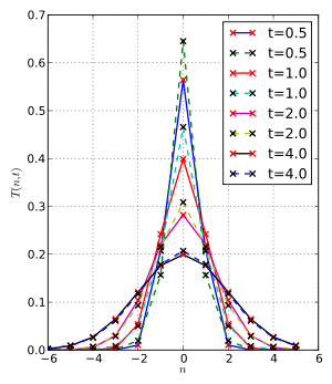The ideal discrete Gaussian kernel (red) compared with sampled ordinary Gaussian (black, dashed), for scales t = [0.5,1,2,4]

A more refined approach is to convolve the original signal by the discrete Gaussian kernel T(n,t)^[1][2]

$L(x, t) = \sum_{n=-\infty}^{\infty} f(x-n) \, T(n, t)$

where

$T(n, t) = e^{-t} I_n(t)\,$

and I_n(t) denotes the modified Bessel functions of integer order. This is the discrete analog of the continuous Gaussian in that it is the solution to the discrete diffusion equation (discrete space, continuous time), just as the continuous Gaussian is the solution to the continuous diffusion equation.

This filter can be truncated in the spatial domain as for the sampled Gaussian

$L(x, t) = \sum_{n=-M}^{M} f(x-n) \, T(n, t)$

or can be implemented in the Fourier domain using a closed-form expression for its discrete-time Fourier transform:

$\hat{T}(\theta, t) = \sum_{n=-\infty}^{\infty} T(n, t) \, e^{-i \theta n} = e^{t(\cos \theta - 1)}$.

With this frequency-domain approach, the scale-space properties transfer exactly to the discrete domain, or with excellent approximation using periodic extension and a suitably long discrete Fourier transform to approximate the discrete-time Fourier transform of the signal being smoothed. Moreover, higher-order derivative approximations can be computed in a straightforward manner (and preserving scale-space properties) by applying small support central difference operators to the discrete scale-space representation.^[3]

As with the sampled Gaussian, a plain truncation of the infinite impulse response will in most cases be a sufficient approximation for small values of ε, while for larger values of ε it is better to use either a decomposition of the discrete Gaussian into a cascade of generalized binomial filters or alternatively to construct a finite approximate kernel by multiplying by a window function. If ε has been chosen too large such that effects of the truncation error begin to appear (for example as spurious extrema or spurious responses to higher-order derivative operators), then the options are to decrease the value of ε such that a larger finite kernel is used, with cutoff where the support is very small, or to use a tapered window.

Recursive filters

Scale-space kernels. Ideal discrete gaussian based on bessel functions (red), and two-pole-pair forward/backward recursive smoothing filters (blue) with poles as described in the text. Top shows individual kernels, and bottom is their cumulative convolution with each other; t = [0.5,1,2,4].

Since computational efficiency is often important, low-order recursive filters are often used for scale-space smoothing. For example, Young and van Vliet^[4] use a third-order recursive filter with one real pole and a pair of complex poles, applied forward and backward to make a sixth-order symmetric approximation to the Gaussian with low computational complexity for any smoothing scale.

By relaxing a few of the axioms, Lindeberg^[1] concluded that good smoothing filters would be "normalized Pólya frequency sequences", a family of discrete kernels that includes all filters with real poles at 0 < Z < 1 and/or Z > 1, as well as with real zeros at Z < 0. For symmetry, which leads to approximate directional homogeneity, these filters must be further restricted to pairs of poles and zeros that lead to zero-phase filters.

To match the transfer function curvature at zero frequency of the discrete Gaussian, which ensures an approximate semi-group property of additive t, two poles at $Z = 1 + {2 / t} - \sqrt{(1 + {2 / t})^2 - 1}$ can be applied forward and backwards, for symmetry and stability. This filter is the simplest implementation of a normalized Pólya frequency sequence kernel that works for any smoothing scale, but it is not as excellent an approximation to the Gaussian as Young and van Vliet's filter, which is not normalized Pólya frequency sequence, due to its complex poles.

The transfer function H₁ of a symmetric pole-pair recursive filter is closely related to the discrete-time Fourier transform of the discrete Gaussian kernel via first-order approximation of the exponential:

$\hat{T}(\theta, t) = {1 \over e^{t(1 - \cos \theta)}} \approx {1 \over {1 +t(1 - \cos \theta)}} = H_1(\theta, t)$

where the t parameter here is related to the stable pole position Z = p via t = 2p / (1 − p)².

Furthermore, such filters with N pairs of poles, such as the two pole pairs illustrated in this section, are an even better approximation to the exponential:

${1 \over {(1 +t(1 - \cos \theta)/N)^N}} = H_N(\theta, t)$

where the stable pole positions are adjusted by solving t / N = 2p / (1 − p)².

The impulse responses of these filters are not very close to gaussian unless more than two pole pairs are used. However, even with only one or two pole pairs per scale, a signal successively smoothed at increasing scales will be very close to a gaussian-smoothed signal. The semi-group property is poorly approximated when too few pole pairs are used.

Scale-space axioms that are still satisfied by these filters are:

• linearity
• shift invariance (integer shifts)
• non-creation of local extrema (zero-crossings) in one dimension
• non-enhancement of local extrema in any number of dimensions
• positivity
• normalization

The following are only approximately satisfied, the approximation being better for larger numbers of pole pairs:

• existence of an infinitesimal generator A (the infinitesimal generator of the discrete Gaussian, or a filter approximating it, approximately maps a recursive filter response to one of infinitesimally larger t )
• the semi-group structure with the associated cascade smoothing property (this property is approximated by considering kernels to be equivalent when they have the same t value, even if they are not quite equal)
• rotational symmetry
• scale invariance

This recursive filter method and variations to compute both the Gaussian smoothing as well as Gaussian derivatives has been described by several authors.^[4][5][6][7] Tan et al. have analyzed and compared some of these approaches, and have pointed out that the Young and van Vliet filters are a cascade (multiplication) of forward and backward filters, while the Deriche and the Jin et al. filters are sums of forward and backward filters.^[8]

At fine scales, the recursive filtering approach as well as other separable approaches are not guaranteed to give the best possible approximation to rotational symmetry, so non-separable implementations for two-dimensional images may be considered as an alternative.

When computing several derivatives in the N-jet simultaneously, discrete scale-space smoothing with the discrete analogue of the Gaussian kernel, or with a recursive filter approximation, followed by small support difference operators, may be both faster and more accurate than computing recursive approximations of each derivative operator.

Finite-impulse-response (FIR) smoothers

For small scales, a low-order FIR filter may be a better smoothing filter than a recursive filter. The symmetric 3-kernel $[ t/2,\ 1-t,\ t/2]$, for $t \le 0.5$ smooths to a scale of t using a pair of real zeros at Z < 0, and approaches the discrete Gaussian in the limit of small t. In fact, with infinitesimal t, either this two-zero filter or the two-pole filter with poles at Z = t / 2 and Z = 2 / t can be used as the infinitesimal generator for the discrete Gaussian kernels described above.

The FIR filter's zeros can be combined with the recursive filter's poles to make a general high-quality smoothing filter. For example, if the smoothing process is to always apply a biquadratic (two-pole, two-zero) filter forward then backwards on each row of data (and on each column in the 2D case), the poles and zeros can each do a part of the smoothing. The zeros limit out at t = 0.5 per pair (zeros at Z = –1), so for large scales the poles do most of the work. At finer scales, the combination makes an excellent approximation to the discrete Gaussian if the poles and zeros each do about half the smoothing. The t values for each portion of the smoothing (poles, zeros, forward and backward multiple applications, etc.) are additive, in accordance with the approximate semi-group property.

Z-plane locations of four poles (X) and four zeros (circles) for a smoothing filter using forward/backward biquad to smooth to a scale t = 2, with half the smoothing from the poles and half from the zeros. The zeros are all at Z = –1; the poles are at Z = 0.172 and Z = 5.83. The poles outside the unit circle are implemented by filtering backwards with the stable poles.

The FIR filter transfer function is closely related to the discrete Gaussian's DTFT, just as was the recursive filter's. For a single pair of zeros, the transfer function is

$\hat{T}(\theta, t) = e^{-t(1 - \cos \theta)} \approx {1 -t(1 - \cos \theta)} = F_1(\theta, t)$

where the t parameter here is related to the zero positions Z = z via t = − 2z / (1 − z)², and we require $t \le 0.5$ to keep the transfer function non-negative.

Furthermore, such filters with N pairs of zeros, are an even better approximation to the exponential and extend to higher values of t :

${(1 -t(1 - \cos \theta)/N)^N} = F_N(\theta, t)\,$

where the stable zero positions are adjusted by solving t / N = − 2z / (1 − z)².

These FIR and pole-zero filters are valid scale-space kernels, satisfying the same axioms as the all-pole recursive filters.

Real-time implementation within pyramids and discrete approximation of scale-normalized derivatives

Regarding the topic of automatic scale selection based on normalized derivatives, pyramid approximations are frequently used to obtain real-time performance^[9][10][11]. The appropriateness of approximating scale-space operations within a pyramid originates from the fact that repeated cascade smoothing with generalized binomial kernels leads to equivalent smoothing kernels that under reasonable conditions approach the Gaussian. Furthermore, the binomial kernels (or more generally the class of generalized binomial kernels) can be shown to constitute the unique class of finite-support kernels that guarantee non-creation of local extrema or zero-crossings with increasing scale (see the article on multi-scale approaches for details). Special care may, however, need to be taken to avoid discretization artifacts.

Other multi-scale approaches

For one-dimensional kernels, there is a well-developed theory of multi-scale approaches, concerning filters that do not create new local extrema or new zero-crossings with increasing scales. For continuous signals, filters with real poles in the s-plane are within this class, while for discrete signals the above-described recursive and FIR filters satisfy these criteria. Combined with the strict requirement of a continuous semi-group structure, the continuous Gaussian and the discrete Gaussian constitute the unique choice for continuous and discrete signals.

There are many other multi-scale signal processing, image processing and data compression techniques, using wavelets and a variety of other kernels, that do not exploit or require the same requirements as scale-space descriptions do; that is, they do not depend on a coarser scale not generating a new extremum that was not present at a finer scale (in 1-D) or non-enhancement of local extrema between adjacent scale levels (in any number of dimensions).

See also

• scale-space
• pyramid (image processing)
• multi-scale approaches
• Gaussian filter

References

1. ^ ^{a b} Lindeberg, T., "Scale-space for discrete signals," PAMI(12), No. 3, March 1990, pp. 234-254.
2. ^ R.A. Haddad and A.N. Akansu, "A Class of Fast Gaussian Binomial Filters for Speech and Image Processing," IEEE Transactions on Acoustics, Speech and Signal Processing, vol. 39, pp 723-727, March 1991.
3. ^ Lindeberg, T. Discrete derivative approximations with scale-space properties: A basis for low-level feature extraction, J. of Mathematical Imaging and Vision, 3(4), pp. 349--376, 1993.
4. ^ ^{a b} Ian T. Young and Lucas J. van Vliet (1995). "Recursive implementation of the Gaussian filter". Signal Processing (Elsevier) 44 (2): pp. 139–151. doi:10.1016/0165-1684(95)00020-E. http://citeseer.ist.psu.edu/young95recursive.html. 
5. ^ Deriche, R: Recursively implementing the Gaussian and its derivatives, INRIA Research Report 1893, 1993.
6. ^ Richard F. Lyon. "Speech recognition in scale space," Proc. of 1987 ICASSP. San Diego, March, pp. 29.3.14, 1987.
7. ^ Jin, JS, Gao Y. "Recursive implementation of LoG Filtering". Real-Time Imaging 1997;3:59–65.
8. ^ . Sovira Tan, Jason L. Dale, and Alan Johnston (2003). "Performance of three recursive algorithms for fast space-variant Gaussian filtering". Real-Time Imaging 9 (3): 215–228. doi:10.1016/S1077-2014(03)00040-8. 
9. ^ Lindeberg, Tony and Bretzner, Lars (2003). "Real-time scale selection in hybrid multi-scale representations". Proc. Scale-Space'03, Springer Lecture Notes in Computer Science. Lecture Notes in Computer Science 2695: 148–163. doi:10.1007/3-540-44935-3_11. ISBN 978-3-540-40368-5. http://www.nada.kth.se/cvap/abstracts/cvap279.html. 
10. ^ Crowley, J, Riff O: Fast computation of scale normalised Gaussian receptive fields, Proc. Scale-Space'03, Isle of Skye, Scotland, Springer Lecture Notes in Computer Science, volume 2695, 2003.
11. ^ Lowe, D. G., “Distinctive image features from scale-invariant keypoints”, International Journal of Computer Vision, 60, 2, pp. 91-110, 2004.