Dinic's algorithm

Dinic's algorithm is a strongly polynomial algorithm for computing the maximum flow in a flow network, conceived in 1970 by Israeli (formerly Soviet) computer scientist Yefim Dinitz. The algorithm runs in O(V²E) time and is similar to the Edmonds–Karp algorithm, which runs in O(VE²) time, in that it uses shortest augmenting paths. The introduction of the concepts of the level graph and blocking flow enable Dinic's algorithm to achieve its performance.

Definition

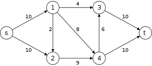
Let G = ((V,E),c,s,t) be a network with c(u,v) and f(u,v) the capacity and the flow of the edge (u,v) respectively.

The residual capacity is a mapping $c_f : V\times V \to R^+$ defined as,

1. if $(u,v)\in E$,

   c_f(u,v) = c(u,v) − f(u,v)

   c_f(v,u) = f(u,v)

2. c_f(u,v) = 0 otherwise.

The residual graph is the graph $G_f = ((V, E_f), c_f|_{E_f}, s, t)$, where

$E_f = \{(u,v)\in V \times V : c_f(u,v) > 0\}$.

An augmenting path is an s − t path in the residual graph G_f.

Define $\operatorname{dist}(v)$ to be the length of the shortest path from s to v in G_f. Then the level graph of G_f is the graph $G_L = (V, E_L, c_f|_{E_L}, s,t)$, where

$E_L = \{(u,v)\in E_f : \operatorname{dist}(v) = \operatorname{dist}(u) + 1\}$.

A blocking flow is an s − t flow f such that the graph G' = (V,E_L',s,t) with $E_L' = \{(u,v) : f(u,v) < c_f|_{E_L}(u,v)\}$ contains no s − t path.

Algorithm

Dinic's Algorithm

Input: A network G = ((V,E),c,s,t).

Output: An s − t flow f of maximum value.

1. Set f(e) = 0 for each $e\in E$.
2. Construct G_L from G_f of G. If $\operatorname{dist}(t) = \infty$, stop and output f.
3. Find a blocking flow $f\;'$ in G_L.
4. Augment flow $\ f$ by $f\;'$ and go back to step 2.

Analysis

It can be shown that the number of edges in each blocking flow increases by at least 1 each time and thus there are at most n − 1 blocking flows in the algorithm, where n is the number of vertices in the network. The level graph G_L can be constructed by Breadth-first search in O(E) time and a blocking flow in each level graph can be found in O(VE) time. Hence, the running time of Dinic's algorithm is O(V²E).

Using a data structure called dynamic trees, the running time of finding a blocking flow in each phase can be reduced to O(Elog V) and therefore the running time of Dinic's algorithm can be improved to O(VElog V).

Special cases

In networks with unit capacities, a much stronger time bound holds. Each blocking flow can be found in O(E) time, and it can be shown that the number of phases does not exceed $O(\sqrt{E})$ and O(V^{2 / 3}). Thus the algorithm runs in O(min(V^{2 / 3},E^{1 / 2})E) time.

In networks arising during the solution of bipartite matching problem, the number of phases is bounded by $O(\sqrt{V})$, therefore leading to the $O(\sqrt{V} E)$ time bound. The resulting algorithm is also known as Hopcroft–Karp algorithm. More generally, this bound holds for any unit network — a network in which each vertex, except for source and sink, either has a single entering edge of capacity one, or a single outgoing edge or capacity one, and all other capacities are arbitrary integers.^[1]

Example

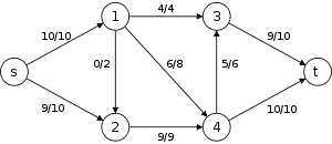
The following is a simulation of the Dinic's algorithm. In the level graph G_L, the vertices with labels in red are the values $\operatorname{dist}(v)$. The paths in blue form a blocking flow.

	G	Gf	GL
1.
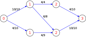
	The blocking flow consists of {s,1,3,t} with 4 units of flow, {s,1,4,t} with 6 units of flow, and {s,2,4,t} with 4 units of flow. Therefore the blocking flow is of 14 units and the value of flow | f | is 14. Note that each augmenting path in the blocking flow has 3 edges.
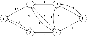
2.
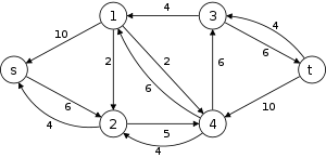
	The blocking flow consists of {s,2,4,3,t} with 5 units of flow. Therefore the blocking flow is of 5 units and the value of flow | f | is 14 + 5 = 19. Note that each augmenting path has 4 edges.
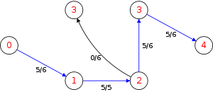
3.
	Since t cannot be reached in Gf. The algorithm terminates and returns a flow with maximum value of 19. Note that in each blocking flow, the number of edges in the augmenting path increases by at least 1.

History

Dinic's algorithm was published in 1970 by former Russian Computer Scientist Yefim (Chaim) A. Dinitz , who is today a member of the Computer Science department at Ben-Gurion University of the Negev (Israel), earlier than the Edmonds–Karp algorithm, which was published in 1972 but was discovered earlier. They independently showed that in the Ford–Fulkerson algorithm, if each augmenting path is the shortest one, the length of the augmenting paths is non-decreasing.

See also

• Ford–Fulkerson algorithm
• Maximum flow problem

Notes

1. ^ Tarjan 1983, p. 102.

References

• Yefim Dinitz (2006). "Dinitz' Algorithm: The Original Version and Even's Version". In Oded Goldreich, Arnold L. Rosenberg, and Alan L. Selman. Theoretical Computer Science: Essays in Memory of Shimon Even. Springer. pp. 218–240. ISBN 978-3540328803. http://www.cs.bgu.ac.il/~dinitz/Papers/Dinitz_alg.pdf. 
• Tarjan, R. E. (1983). Data structures and network algorithms. 
• B. H. Korte, Jens Vygen (2008). "8.4 Blocking Flows and Fujishige's Algorithm". Combinatorial Optimization: Theory and Algorithms (Algorithms and Combinatorics, 21). Springer Berlin Heidelberg. pp. 174–176. ISBN 978-3-540-71844-4.