Modularity (networks)

For other uses, see Modularity.

Modularity is one measure of the structure of networks or graphs. It measures the strength of division of a network into modules (also called groups, clusters or communities). Networks with high modularity have dense connections between the nodes within modules but sparse connections between nodes in different modules. Modularity is often used in optimisation methods for detecting community structure in networks.

Motivation

Many scientifically important problems can be represented and empirically studied using networks. For example, biological and social patterns, the world-wide web, metabolic networks, food webs, neural networks and pathological networks are a few examples of real world problems that can be mathematically represented and topologically studied to reveal some unexpected structural features ^[1]. Most of these networks possess a certain community structure that has substantial importance in building an understanding regarding the dynamics of the network. For instance, a closely connected social community will imply a faster rate of transmission of information or rumor among them than a loosely connected community. Thus, if a network is represented by a number of individual nodes connected by links which signify a certain degree of interaction between the nodes, communities are defined as groups of densely interconnected nodes that are only sparsely connected with the rest of the network. Hence, it may be imperative to identify the communities in networks since the communities may have quite different properties such as node degree, clustering coefficient, betweenness, centrality ^[2]. etc, from that of the average network. Modularity is one such measure, which when maximized; it leads to the appearance of communities in a given network.

Definition

Modularity is the fraction of the edges that fall within the given groups minus the expected such fraction if edges were distributed at random. The value of the modularity lies in the range [−1,1]. It is positive if the number of edges within groups exceeds the number expected on the basis of chance. For a given division of the network's vertices into some modules, modularity reflects the concentration of nodes within modules compared with random distribution of links between all nodes regardless of modules.

There are different methods for calculating modularity.^[1] In the most common version of the concept, the randomization of the edges is done so as to preserve the degree of each vertex. Let us consider a graph with n nodes vertices and m edges edges such that the graph can be partitioned into 2 communities using a membership variable s. If a node i belongs to community 1, s _i =1, or if i belongs to community 2, s_i=-1. Let the adjacency matrix for the network be represented by A_ij adjacency matrix , where A_ij =0 signifies no edge (no interaction) between node i and j and A_ij =1 signifies an existing edge. Also for simplicity we consider an undirected network. Thus A_ij =A_ji . (It is important to note that multiple edges may exist between 2 nodes and here we assess the simplest case).

Modularity Q=(Fraction of edges that fall within group 1 or 2) - (Expected number if edges within group 1 and 2 for a random graph with same node degree distribution as the given network). (1)

In (1), the second term on the right hand side shall be computed using the concept of Configuration Models ^[3]. The configuration model is a randomized realization of a particular network. Given a network with n nodes, where each node i has a node degree ki, the configuration model cuts each edge into 2 halves, and then each half edge, called a stub, is rewired randomly with any other stub in the network even allowing self loops. Thus, even though the node degree distribution of the graph remains intact, the configuration model results in a completely random network.

Let the total number of stubs be l_n

$l_{n}= \sum_{i}^{n} k_{i} =2m$

Now, if we randomly select two nodes i and j with node degrees k_i and k_j respectively and rewire the stubsfor these 2 nodes, then,

Expected [Full edges between i and j] = (Full edges between i and j)/(Total number of rewirings possible) (2)

Total number of rewritings possible = number of stubs remaining after choosing a particular stub = l_n-1= l _n for large n

Thus, Expected [Number of full edges between i and j]=(k_i* k_j)/l_n =(k_i k_j)/2m.

Hence, the actual number of edges between i and j minus expected number of edges between them is A_ij-(k_i k_j )/2m. Thus using ^[1]

$Q = \frac{1}{4m} \sum_{ij} \left[ A_{ij} - \frac{k_i*k_j}{2m} \right] (s_{i} s_{j}+1) (3)$

It is important to note that (3) holds good for partitioning into 2 communities only. Hierarchical partitioning (i.e. partitioning into 2 communities, then the 2 sub-communities further partitioned into 2 smaller sub communities only to maximize Q) is a possible approach to identify multiple communities in a network. Additionally, (3) can be generalized for partitioning a network into c communities. ^[4].

$Q = \sum_{ij} \left[ \frac {A_{ij}}{2m} - \frac{k_i*k_j}{(2m)(2m)} \right] \frac{(s_{i} s_{j}+1)}{2} =\sum_{i=1}^{c} (e_{ii}-a_{i}^2) (4)$

where e_ii is the fraction of edges with both end vertices in the same community i.

$e_{ii}= \sum_{ij} \frac{A_{ij}}{2m} \delta(i,j)$

and a_i is the fraction of edges with at least one end vertex in community i.

$a_i=\frac{k_i}{2m} = \sum_{j} e_{ij}$

Example of multiple community detection

We consider an undirected network with 10 nodes and 12 edges and the following adjacency matrix.

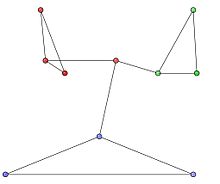Fig 1. Sample Network corresponding to the Adjacency matrix with 10 nodes, 12 edges.

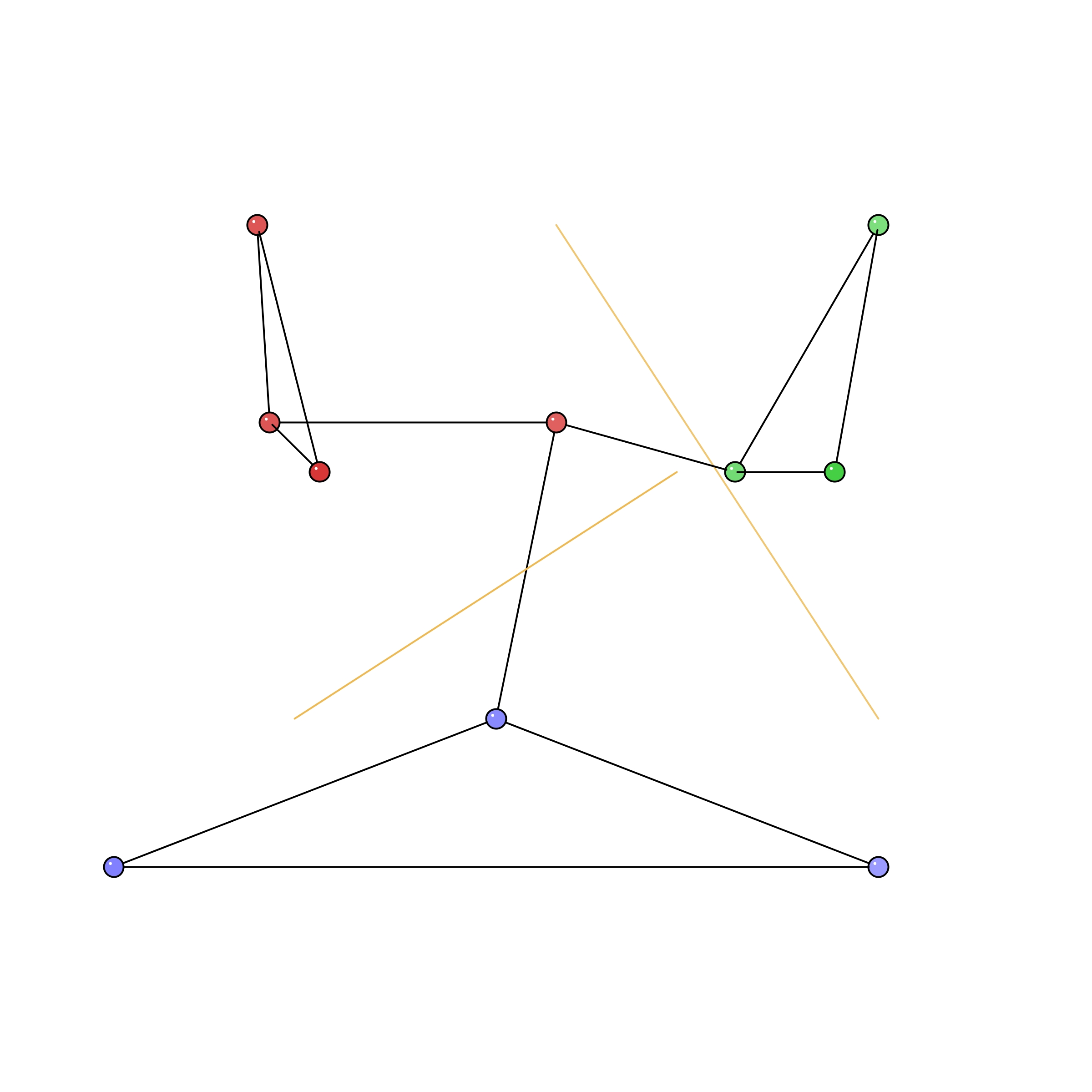
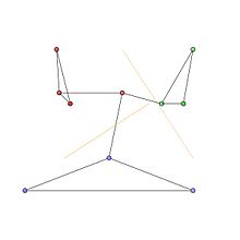Fig 2. Network partitions that maximize Q. Maximum Q=0.4985

Node ID	1	2	3	4	5	6	7	8	9	10
1	0	1	1	0	0	0	0	0	0	1
2	1	0	1	0	0	0	0	0	0	0
3	1	1	0	0	0	0	0	0	0	0
4	0	0	0	0	1	1	0	0	0	1
5	0	0	0	1	0	1	0	0	0	0
6	0	0	0	1	1	0	0	0	0	0
7	0	0	0	0	0	0	0	1	1	1
8	0	0	0	0	0	0	1	0	1	0
9	0	0	0	0	0	0	1	1	0	0
10	1	0	0	1	0	0	1	0	0	0

The communities in the graph are represented by the red, green and blue node clusters in Fig 1. The optimal community partitions are depicted in Fig 2.

Matrix formulation

An alternative formulation of the modularity, useful particularly in spectral optimization algorithms, is as follows.^[1] Define S_ir to be 1 if vertex i belongs to group r and zero otherwise. Then

δ(ci,cj) =	∑	SirSjr
	r

and hence

$Q = \frac{1}{4m} \sum_{ij} \sum_r \left[ A_{ij} - \frac{k_i k_j}{2m} \right] S_{ir} S_{jr} = \frac{1}{4m} \mathrm{Tr}(\mathbf{S}^\mathrm{T}\mathbf{BS}),$

where S is the (non-square) matrix having elements S_ir and B is the so-called modularity matrix, which has elements

$B_{ij} = A_{ij} - \frac{k_i k_j}{2m}.$

All rows and columns of the modularity matrix sum to zero, which means that the modularity of an undivided network is also always zero.

For networks divided into just two communities, one can alternatively define s_i = ±1 to indicate the community to which node i belongs, which then leads to

$Q = {1\over 4m} \sum_{ij} B_{ij} s_i s_j = {1\over 4m} \mathbf{s}^\mathrm{T}\mathbf{Bs},$

where s is the column vector with elements s_i.^[1]

This function has the same form as the Hamiltonian of an Ising spin glass, a connection that has been exploited to create simple computer algorithms, for instance using simulated annealing, to maximize the modularity. The general form of the modularity for arbitrary numbers of communities is equivalent to a Potts spin glass and similar algorithms can be developed for this case also.^[5]

Resolution limit

Modularity compares the number of edges inside a cluster with the expected number of edges that one would find in the cluster if the network were a random network with the same number of nodes and where each node keeps its degree, but edges are otherwise randomly attached. This random null model implicitly assumes that each node can get attached to any other node of the network. Such assumption is however unreasonable if the network is very large, as the horizon of a node includes a small part of the network, ignoring most of it. Moreover, this implies that the expected number of edges between two groups of nodes decreases if the size of the network increases. So, if a network is large enough, the expected number of edges between two groups of nodes in modularity's null model may be smaller than one. If this happens, a single edge between the two clusters would be interpreted by modularity as a sign of a strong correlation between the two clusters, and optimizing modularity would lead to the merge of the two clusters, independently of the clusters' features. So, even weakly interconnected complete graphs, which have the highest possible density of internal edges, and represent the best identifiable communities, would be merged by modularity optimization if the network is sufficiently large.^[6] For this reason, optimizing modularity in large networks would fail to resolve small communities, even when they are well defined. This bias is inevitable for methods like modularity optimization, which rely on a global null model.^[7]

Multiresolution methods

There are two main approaches to solve the resolution limit within the modularity context: the addition of a resistance r to every node, in the form of a self-loop, which increases (r>0) or decreases (r<0) the aversion of nodes to form communities;^[8] or the addition of a parameter γ>0 in front of the null-case term in the definition of modularity, which controls the relative importance between internal links of the communities and the null model.^[5] Optimizing modularity for values of these parameters in their respective appropriate ranges, it is possible to recover the whole mesoscale of the network, from the macroscale in which all nodes belong to the same community, to the microscale in which every node forms its own community, thus the name multiresolution methods.

See also

• Complex network
• Community structure

References

1. ^ ^{a b c d e} Newman, M. E. J. (2006). "Modularity and community structure in networks". PROCEEDINGS- NATIONAL ACADEMY OF SCIENCES USA 103 (23): 8577–8696. doi:10.1073/pnas.0601602103. 
2. ^ Newman, M. E. J. (2007). Palgrave Macmillan, Basingstoke. ed. "Mathematics of networks". The New Palgrave Encyclopedia of Economics. 
3. ^ Remco van der Hofstad (2009). "7". Random Graphs and Complex Networks. 
4. ^ Clauset, Aaron and Newman, M. E. J. and Moore, Cristopher (2004). "Finding community structure in very large networks". Phys. Rev. E 70 (6): 066111. doi:10.1103/PhysRevE.70.066111. 
5. ^ ^{a b} Joerg Reichardt and Stefan Bornholdt (2006). "Statistical mechanics of community detection". Physical Review E 74 (1): 016110. arXiv:cond-mat/0603718. Bibcode 2006PhRvE..74a6110R. doi:10.1103/PhysRevE.74.016110. 
6. ^ Santo Fortunato and Marc Barthelemy (2007). "Resolution limit in community detection". Proceedings of the National Academy of Science of the USA 104 (1): 36–41. arXiv:physics/0607100. Bibcode 2007PNAS..104...36F. doi:10.1073/pnas.0605965104. PMC 1765466. PMID 17190818. http://www.pnas.org/content/104/1/36.abstract. 
7. ^ J.M. Kumpula, J. Saramäki, K. Kaski , and J. Kertész (2007). "Limited resolution in complex network community detection with Potts model approach". The European Physical Journal B 56 (1): 41–45. arXiv:cond-mat/0610370. Bibcode 2007EPJB...56...41K. doi:10.1140/epjb/e2007-00088-4. 
8. ^ Alex Arenas, Alberto Fernández and Sergio Gómez (2008). "Analysis of the structure of complex networks at different resolution levels". New Journal of Physics 10 (5): 053039. arXiv:physics/0703218. Bibcode 2008NJPh...10e3039A. doi:10.1088/1367-2630/10/5/053039. 

External links

• M. E. J. Newman (2006). "Modularity and community structure in networks". Proc. Natl. Acad. Sci. USA 103 (23): 8577–8582. arXiv:physics/0602124. Bibcode 2006PNAS..103.8577N. doi:10.1073/pnas.0601602103. PMC 1482622. PMID 16723398. http://www.pnas.org/content/103/23/8577.full. Retrieved 2008-07-11.