Deutsch–Jozsa algorithm

The Deutsch–Jozsa algorithm is a quantum algorithm, proposed by David Deutsch and Richard Jozsa in 1992^[1] with improvements by Richard Cleve, Artur Ekert, Chiara Macchiavello, and Michele Mosca in 1998.^[2] Although it is of little practical use, it is one of the first examples of a quantum algorithm that is exponentially faster than any possible deterministic classical algorithm.

Problem statement

In the Deutsch-Jozsa problem, we are given a black box quantum computer known as an oracle that implements the function $f:\{0,1\}^n\rightarrow \{0,1\}$. We are promised that the function is either constant (0 on all inputs or 1 on all inputs) or balanced^[3] (returns 1 for half of the input domain and 0 for the other half); the task then is to determine if f is constant or balanced by using the oracle.

Motivation

It has been shown there are random string query oracles relative to which P and NP are separated. In analogy, we can have oracles relative to which EQP and P are separated. This tells us nothing about BPP or BQP, though.

For the Deutsch-Jozsa oracle, P and BPP are also separated. This is because in the worst-case scenario, which can be extremely unlikely, deterministic pseudorandom queries can be anticipated and conspired against. Please note the seed can't be chosen randomly.

Simon's algorithm is with respect to an oracle separating BQP from BPP.

Classical solution

For a conventional deterministic algorithm where n is number of bits/qubits, 2^{n − 1} + 1 evaluations of f will be required in the worst case. To prove that f is constant, just over half the set of outputs must be evaluated and found to be identical (remembering that the function is guaranteed to be either balanced or constant, not somewhere in between). The best case occurs where the function is balanced and the first two output values that happen to be selected are different. For a conventional randomized algorithm, a constant k evaluations of the function suffices to produce the correct answer with a high probability (failing with probability $\epsilon \leq 1/2^{k-1}$). However, k = 2^{n − 1} + 1 evaluations are still required if we want an answer that is always correct. The Deutsch-Jozsa quantum algorithm produces an answer that is always correct with a single evaluation of f.

History

The Deutsch–Jozsa Algorithm generalizes earlier (1985) work by David Deutsch, which provided a solution for the simple case.
Specifically we were given a boolean function whose input is 1 bit, $f: \{0,1\} \rightarrow \{0,1\}$ and asked if it is constant.^[4]

The algorithm as Deutsch had originally proposed it was not, in fact, deterministic. The algorithm was successful with a probability of one half. In 1992, Deutsch and Jozsa produced a deterministic algorithm which was generalized to a function which takes n bits for its input. Unlike Deutsch's Algorithm, this algorithm required two function evaluations instead of only one.

Further improvements to the Deutsch–Jozsa algorithm were made by Cleve et al.,^[2] resulting in an algorithm that is both deterministic and requires only a single query of f. This algorithm is still referred to as Deutsch–Jozsa algorithm in honour of the groundbreaking techniques they employed.^[2]

The Deutsch–Jozsa algorithm provided inspiration for Shor's algorithm and Grover's algorithm, two of the most revolutionary quantum algorithms.^[5][6]

Decoherence

For the Deutsch–Jozsa algorithm to work, the oracle computing f(x) from x has to be a quantum oracle which doesn't decohere x. It also mustn't leave any copy of x lying around at the end of the oracle call.

Deutsch's Algorithm

Deutsch's algorithm is a special case of the general Deutsch–Jozsa algorithm. We need to check the condition f(0) = f(1). It is equivalent to check $f(0)\oplus f(1)$ (where $\oplus$ is addition modulo 2), if zero, then f is constant, otherwise f is not constant.

We begin with the two-qubit state $|0\rangle |1\rangle$ and apply a Hadamard transform to each qubit. This yields

$\frac{1}{2}(|0\rangle + |1\rangle)(|0\rangle - |1\rangle).$

We are given a quantum implementation of the function f which maps $|x\rangle |y\rangle$ to $|x\rangle |f(x)\oplus y\rangle$. Applying this function to our current state we obtain

$\frac{1}{2}(|0\rangle(|f(0)\oplus 0\rangle - |f(0)\oplus 1\rangle) + |1\rangle(|f(1)\oplus 0\rangle - |f(1)\oplus 1\rangle))$

$=\frac{1}{2}((-1)^{f(0)}|0\rangle(|0\rangle - |1\rangle) + (-1)^{f(1)}|1\rangle(|0\rangle - |1\rangle))$

$=(-1)^{f(0)}\frac{1}{2}(|0\rangle + (-1)^{f(0)\oplus f(1)}|1\rangle)(|0\rangle - |1\rangle).$

We ignore the last bit and the global phase and therefore have the state

$\frac{1}{\sqrt{2}}(|0\rangle + (-1)^{f(0)\oplus f(1)}|1\rangle).$

Applying a Hadamard transform to this state we have

$\frac{1}{2}(|0\rangle + |1\rangle + (-1)^{f(0)\oplus f(1)}|0\rangle - (-1)^{f(0)\oplus f(1)}|1\rangle)$

$=\frac{1}{2}((1 +(-1)^{f(0)\oplus f(1)})|0\rangle + (1-(-1)^{f(0)\oplus f(1)})|1\rangle).$

Obviously $f(0)\oplus f(1)=0$ if and only if we measure a zero. Therefore the function is constant if and only if we measure a zero.

Deutsch–Jozsa algorithm

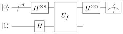The Deutsch-Jozsa algorithm's quantum circuit

The algorithm begins with the n+1 bit state $|0\rangle^{\otimes n} |1\rangle$. That is, the first n bits are each in the state $|0\rangle$ and the final bit is $|1\rangle$. A Hadamard transformation is applied to each bit to obtain the state

$\frac{1}{\sqrt{2^{n+1}}}\sum_{x=0}^{2^n-1} |x\rangle (|0\rangle - |1\rangle )$.

We have the function f implemented as quantum oracle. The oracle maps the state $|x\rangle|y\rangle$ to $|x\rangle|y\oplus f(x) \rangle$. Applying the quantum oracle gives

$\frac{1}{\sqrt{2^{n+1}}}\sum_{x=0}^{2^n-1} |x\rangle (|f(x)\rangle - |1\oplus f(x)\rangle )$.

For each x, f(x) is either 0 or 1. A quick check of these two possibilities yields

$\frac{1}{\sqrt{2^{n+1}}}\sum_{x=0}^{2^n-1} (-1)^{f(x)} |x\rangle (|0\rangle - |1\rangle )$.

At this point the last qubit may be ignored. We apply a Hadamard transformation to each qubit to obtain

$\frac{1}{2^n}\sum_{x=0}^{2^n-1} (-1)^{f(x)} \sum_{y=0}^{2^n-1}(-1)^{x\cdot y} |y\rangle= \frac{1}{2^n}\sum_{y=0}^{2^n-1} \left[\sum_{x=0}^{2^n-1}(-1)^{f(x)} (-1)^{x\cdot y}\right] |y\rangle$

where $x\cdot y=x_0 y_0\oplus x_1 y_1\oplus\cdots\oplus x_{n-1} y_{n-1}$ is the sum of the bitwise product.

Finally we examine the probability of measuring $|0\rangle^{\otimes n}$,

$\bigg|\frac{1}{2^n}\sum_{x=0}^{2^n-1}(-1)^{f(x)}\bigg|^2$

which evaluates to 1 if f(x) is constant (constructive interference) and 0 if f(x) is balanced (destructive interference).

References

1. ^ David Deutsch and Richard Jozsa (1992). "Rapid solutions of problems by quantum computation". Proceedings of the Royal Society of London A 439: 553. Bibcode 1992RSPSA.439..553D. doi:10.1098/rspa.1992.0167. 
2. ^ ^{a b c} R. Cleve, A. Ekert, C. Macchiavello, and M. Mosca (1998). "Quantum algorithms revisited". Proceedings of the Royal Society of London A 454: 339–354. arXiv:quant-ph/9708016. Bibcode 1998RSPSA.454..339C. doi:10.1098/rspa.1998.0164. 
3. ^ Certainty from Uncertainty
4. ^ David Deutsch (1985). "The Church-Turing principle and the universal quantum computer" (PDF). Proceedings of the Royal Society of London A 400: 97. Bibcode 1985RSPSA.400...97D. doi:10.1098/rspa.1985.0070. http://coblitz.codeen.org:3125/citeseer.ist.psu.edu/cache/papers/cs/13701/http:zSzzSzwww.qubit.orgzSzresourcezSzdeutsch85.pdf/deutsch85quantum.pdf. 
5. ^ Lov K. Grover (1996). "A fast quantum mechanical algorithm for database search". Proceedings of the Twenty-Eighth Annual ACM Symposium on Theory of Computing. pp. 212–219. arXiv:quant-ph/9605043. doi:10.1145/237814.237866. 
6. ^ Peter W. Shor (1994). "Algorithms for quantum computation: discrete logarithms and factoring" (PDF). Proceedings of the 35th IEEE Symposium on Foundations of Computer Science. pp. 124–134. doi:10.1109/SFCS.1994.365700. http://citeseer.ist.psu.edu/cache/papers/cs/408/http:zSzzSzwww.research.att.comzSz%7EshorzSzpaperszSzQCalgs.pdf/algorithms-for-quantum-computation.pdf. 

External links

• Deutsch's lecture about Deutsch algorithm
• Implementation of the Deutsch-Jozsa algorithm in the Scala programming language