Generalized mean

In mathematics, a generalized mean, also known as power mean or Hölder mean (named after Otto Hölder), is an abstraction of the Pythagorean means including arithmetic, geometric, and harmonic means.

Definition

If p is a non-zero real number, we can define the generalized mean with exponent p (or power mean with exponent p) of the positive real numbers $x_1,\dots,x_n$ as:

$M_p(x_1,\dots,x_n) = \left( \frac{1}{n} \sum_{i=1}^n x_i^p \right)^{1/p}$

While for p equal to 0 we assume that it's equal to the geometric mean (which is, in fact, the limit of means with exponents approaching zero):

$M_0(x_1, \dots, x_n) = \sqrt[n]{\prod_{i=1}^n x_i}$

Furthermore, for a sequence of positive weights w_i with sum $w=\sum w_i$ we can define weighted power means as follows:

$M_p(x_1,\dots,x_n) = \left( \frac{1}{w}\sum_{i=1}^n w_ix_{i}^p \right)^{1/p}$

$M_0(x_1,\dots,x_n) = \sqrt[w]{\prod_{j=1}^n x_j^{w_j}}$

For the sake of simplicity, we might assume that the weights are normalized so that they sum up to 1 (which can be easily done by dividing each weight by their sum), thus allowing some terms in the above formulae to be omitted:

$M_p(x_1,\dots,x_n) = \left(\sum_{i=1}^n w_ix_{i}^p \right)^{1/p}$

$M_0(x_1,\dots,x_n) = \prod_{i=1}^n x_i^{w_i}$

The unweighted means can be easily produced by assuming that all weights equal 1/n. For exponents equal to positive or negative infinity the means are maximum and minimum, respectively, regardless of weights (and they are actually the limit points for exponents approaching the respective extremes):

$M_\infty (x_1,\dots,x_n)=\max(x_1,\dots,x_n)$

$M_{-\infty}(x_1,\dots,x_n)=\min(x_1,\dots,x_n)$

Properties

• Like most means, the generalized mean is a homogeneous function of its arguments $x_1,\dots,x_n$. That is, if b is a positive real number, then the generalized mean with exponent p of the numbers $b\cdot x_1,\dots, b\cdot x_n$ is equal to b times the generalized mean of the numbers $x_1,\dots, x_n$.
• Like the quasi-arithmetic means, the computation of the mean can be split into computations of equal sized sub-blocks.

$M_p(x_1,\dots,x_{n\cdot k}) = M_p(M_p(x_1,\dots,x_{k}), M_p(x_{k+1},\dots,x_{2\cdot k}), \dots, M_p(x_{(n-1)\cdot k + 1},\dots,x_{n\cdot k}))$

Generalized mean inequality

In general, if p < q, then $M_p(x_1,\dots,x_n) \le M_q(x_1,\dots,x_n)$ and the two means are equal if and only if $x_1 = x_2 = \cdots = x_n$.

It is true for real nonzero p, as well as zero, positive and negative infinity p, as defined above.

This follows from the fact that, for all p in $\mathbb{R}$,

$\frac{\partial M_p(x_1,\dots,x_n)}{\partial p}\geq 0,$

which can be proved using Jensen's inequality. In particular, for $p\in\{-1, 0, 1\}$, the generalized mean inequality implies the Pythagorean means inequality as well as the inequality of arithmetic and geometric means.

Special cases

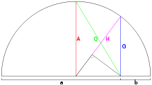A visual depiction of some of the specified cases for n=2.

$\lim_{p\to-\infty} M_p(x_1,\dots,x_n) = \min \{x_1,\dots,x_n\}$	minimum
$M_{-1}(x_1,\dots,x_n) = \frac{n}{\frac{1}{x_1}+\dots+\frac{1}{x_n}}$	harmonic mean
$\lim_{p\to0} M_p(x_1,\dots,x_n) = \sqrt[n]{x_1\cdot\dots\cdot x_n}$	geometric mean
$M_1(x_1,\dots,x_n) = \frac{x_1 + \dots + x_n}{n}$	arithmetic mean
$M_2(x_1,\dots,x_n) = \sqrt{\frac{x_1^2 + \dots + x_n^2}{n}}$	quadratic mean, a.k.a. root mean square
$\lim_{p\to\infty} M_p(x_1,\dots,x_n) = \max \{x_1,\dots,x_n\}$	maximum

Proof of power means inequality

We will prove weighted power means inequality, for the purpose of the proof we will assume without loss of generality that:

$w_i\in (0;1]$

and

$\sum_{i=1}^nw_i=1$

Proof for unweighted power means is easily obtained by substituting $w_i=\frac{1}{n}$.

Equivalence of inequalities between means of opposite signs

Suppose an average between power means with exponents p and q holds:

$\sqrt[p]{\sum_{i=1}^nw_ix_i^p}\leq \sqrt[q]{\sum_{i=1}^nw_ix_i^q}$

then:

$\sqrt[p]{\sum_{i=1}^n\frac{w_i}{x_i^p}}\leq \sqrt[q]{\sum_{i=1}^n\frac{w_i}{x_i^q}}$

We raise both sides to the power of −1 (strictly decreasing function in positive reals):

$\sqrt[-p]{\sum_{i=1}^nw_ix_i^{-p}}=\sqrt[p]{\frac{1}{\sum_{i=1}^nw_i\frac{1}{x_i^p}}}\geq \sqrt[q]{\frac{1}{\sum_{i=1}^nw_i\frac{1}{x_i^q}}}=\sqrt[-q]{\sum_{i=1}^nw_ix_i^{-q}}$

We get the inequality for means with exponents −p and −q, and we can use the same reasoning backwards, thus proving the inequalities to be equivalent, which will be used in some of the later proofs.

Geometric mean

For any q the inequality between mean with exponent q and geometric mean can be transformed in the following way:

$\prod_{i=1}^nx_i^{w_i} \leq \sqrt[q]{\sum_{i=1}^nw_ix_i^q}$

$\sqrt[q]{\sum_{i=1}^nw_ix_i^q}\leq \prod_{i=1}^nx_i^{w_i}$

(the first inequality is to be proven for positive q, and the latter otherwise)

We raise both sides to the power of q:

$\prod_{i=1}^nx_i^{w_i\cdot q} \leq \sum_{i=1}^nw_ix_i^q$

in both cases we get the inequality between weighted arithmetic and geometric means for the sequence $x_i^q$, which can be proved by Jensen's inequality, making use of the fact the logarithmic function is concave:

$\sum_{i=1}^nw_i\log(x_i) \leq \log\left( \sum_{i=1}^nw_ix_i \right)$

$\log \left( \prod_{i=1}^nx_i^{w_i} \right) \leq \log \left( \sum_{i=1}^nw_ix_i \right)$

By applying (strictly increasing) exp function to both sides we get the inequality:

$\prod_{i=1}^nx_i^{w_i} \leq \sum_{i=1}^nw_ix_i$

Thus for any positive q it is true that:

$\sqrt[-q]{\sum_{i=1}^nw_ix_i^{-q}}\leq \prod_{i=1}^nx_i^{w_i} \leq \sqrt[q]{\sum_{i=1}^nw_ix_i^q}$

thus we have proved the inequality between geometric mean and any power mean.

Geometric mean as a limit

Furthermore, we can prove that the geometric mean is the limit of power means for exponent approaching zero. Firstly, we will prove the limit:

$\lim_{p\to0} \frac{\log\left(\sum_{i=1}^nw_ix_i^p\right)}{p}=\sum_{i=1}^nw_i\log(x_i)$

It's easy to conclude that the limits of both the numerator and the denominator are both 0, so we can use L'Hôpital's rule:

$\lim_{p\to 0} \frac{\log\left(\sum_{i=1}^nw_ix_i^p\right)}{p}=\lim_{p\to 0}\frac{1}{\sum_{i=1}^nw_ix_i^p}\cdot\left(\sum_{i=1}^nw_ix_i^p\right)'=$

$=\frac{1}{\sum_{i=1}^nw_i}\cdot \lim_{p\to 0}\sum_{i=1}^n(w_i\cdot\log(x_i)\cdot x_i^p)=\sum_{i=1}^nw_i\log(x_i)$

Then we make use of the exponential function's continuity:

$\begin{align} & \lim_{p \to 0} \sqrt[p]{\sum_{i=1}^nw_ix_i^p}=\lim_{p \to 0} \exp\left(\frac{\log\left(\sum_{i=1}^nw_ix_i^p\right)}{p}\right) \\ & = \exp\left(\lim_{p \to 0} \frac{\log\left(\sum_{i=1}^nw_ix_i^p\right)}{p}\right)=\exp\left(\sum_{i=1}^nw_i\log(x_i)\right)=\prod_{i=1}^nx_i^{w_i} \end{align}$

which was to be proven.

Inequality between any two power means

We are to prove that for any p < q the following inequality holds:

$\sqrt[p]{\sum_{i=1}^nw_ix_i^p}\leq \sqrt[q]{\sum_{i=1}^nw_ix_i^q}$

if p is negative, and q is positive, the inequality is equivalent to the one proved above:

$\sqrt[p]{\sum_{i=1}^nw_ix_i^p}\leq \prod_{i=1}^nx_i^{w_i} \leq\sqrt[q]{\sum_{i=1}^nw_ix_i^q}$

The proof for positive p and q is as follows: Define the following function: $f:{\mathbb R_+}\rightarrow{\mathbb R_+},$ $f(x)=x^{\frac{q}{p}}$. f is a power function, so it does have a second derivative:

$f''(x) = \left(\frac{q}{p} \right) \left( \frac{q}{p}-1 \right)x^{\frac{q}{p}-2},$

which is strictly positive within the domain of f, since q > p, so we know f is convex.

Using this, and the Jensen's inequality we get:

$f \left( \sum_{i=1}^nw_ix_i^p \right) \leq \sum_{i=1}^nw_if(x_i^p)$

$\sqrt[\frac{q}{p}]{\sum_{i=1}^nw_ix_i^p}\leq\sum_{i=1}^nw_ix_i^q$

after raising both side to the power of 1/q (an increasing function, since 1/q is positive) we get the inequality which was to be proven:

$\sqrt[p]{\sum_{i=1}^nw_ix_i^p}\leq\sqrt[q]{\sum_{i=1}^nw_ix_i^q}$

Using the previously shown equivalence we can prove the inequality for negative p and q by substituting them with, respectively, −q and −p, QED.

Minimum and maximum

Minimum and maximum are the limits of power means at, respectively, $- \infty$ and $+\infty$. The proof is as follows:

Suppose without loss of generality that x₁ is the largest, while x_n is the smallest of x_i. First, using the squeeze theorem we will prove that:

$\lim_{p \to \infty}\left(\frac{1}{p}\ln\left(\frac{\sum_{i=1}^nw_ix_i^p}{x_1^p}\right)\right)=0$

It suffices to notice that for positive p the inequalities hold:

$\frac{1}{p}\ln(w_1)=\frac{1}{p}\ln\left(\frac{w_1x_1^p}{x_1^p}\right)\leq\frac{1}{p}\ln\left(\frac{\sum_{i=1}^nw_ix_i^p}{x_1^p}\right)\leq\frac{1}{p}\ln\left(\frac{\sum_{i=1}^nw_ix_1^p}{x_1^p}\right)=\ln(1)=0$

Then, making use of the limit:

$\lim_{p \to \infty}\frac{1}{p}\ln\left(\sum_{i=1}^nw_ix_i^p\right)=\lim_{p \to \infty}\frac{1}{p}\ln\left(x_1^p\cdot\frac{\sum_{i=1}^nw_ix_i^p}{x_1^p}\right)=\lim_{p \to \infty}\left(\frac{\ln(x_1^p)}{p}\right)+\lim_{p \to \infty}\left(\frac{1}{p}\ln\left(\frac{\sum_{i=1}^nw_ix_i^p}{x_1^p}\right)\right)=\ln(x_1)+0=\ln(x_1)$

and finally, we use the fact that the exponential function is continuous:

$\lim_{p \to \infty}\sqrt[p]{\sum_{i=1}^nw_ix_i^p}=\lim_{p \to \infty}\exp\left(\frac{1}{p}\ln\left(\sum_{i=1}^nw_ix_i^p\right)\right)=\exp\left(\lim_{p \to \infty}\frac{1}{p}\ln\left(\sum_{i=1}^nw_ix_i^p\right)\right)=x_1$

Similarly, for negative p:

$\lim_{p \to -\infty}\left(\frac{1}{p}\ln\left(\frac{\sum_{i=1}^nw_ix_n^p}{x_n^p}\right)\right)=0$

since (for p < 0):

$\frac{1}{p}\ln(w_n)=\frac{1}{p}\ln\left(\frac{w_nx_n^p}{x_n^p}\right) \geq\frac{1}{p}\ln\left(\frac{\sum_{i=1}^nw_ix_i^p}{x_n^p}\right)\geq\frac{1}{p}\ln\left(\frac{\sum_{i=1}^nw_ix_n^p}{x_n^p}\right)=\ln(1)=0$

Thus:

$\lim_{p \to-\infty}\frac{1}{p}\ln\left(\sum_{i=1}^nw_ix_i^p\right)=\lim_{p \to -\infty}\left(\frac{\ln(x_n^p)}{p}\right)+\lim_{p \to -\infty}\left(\frac{1}{p}\ln\left(\frac{\sum_{i=1}^nw_ix_i^p}{x_n^p}\right)\right)=\ln(x_n)$

and again, by continuity of the exp function:

$\lim_{p \to-\infty}\sqrt[p]{\sum_{i=1}^nw_ix_i^p}=\exp\left(\lim_{p \to -\infty}\frac{1}{p}\ln\left(\sum_{i=1}^nw_ix_i^p\right)\right)=x_n$

Generalized f-mean

Main article: Generalized ƒ-mean

The power mean could be generalized further to the generalized f-mean:

$M_f(x_1,\dots,x_n) = f^{-1} \left({\frac{1}{n}\cdot\sum_{i=1}^n{f(x_i)}}\right)$

which covers e.g. the geometric mean without using a limit. The power mean is obtained for $f\left(x\right)=x^p$.

Applications

Signal processing

A power mean serves a non-linear moving average which is shifted towards small signal values for small p and emphasizes big signal values for big p. Given an efficient implementation of a moving arithmetic mean called smooth you can implement a moving power mean according to the following Haskell code.

 powerSmooth :: Floating a => ([a] -> [a]) -> a -> [a] -> [a]
 powerSmooth smooth p = map (** recip p) . smooth . map (**p)

• For big p it can serve an envelope detector on a rectified signal.
• For small p it can serve an baseline detector on a mass spectrum.

See also

• Arithmetic mean
• Arithmetic-geometric mean
• Average
• Geometric mean
• Harmonic mean
• Heronian mean
• Inequality of arithmetic and geometric means
• Lehmer mean – also a mean related to powers
• Root mean square

External links

• Power mean at MathWorld
• Examples of Generalized Mean
• A proof of the Generalized Mean on PlanetMath