Optical autocorrelation

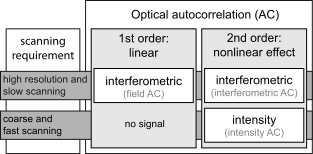Classification of the different kinds of optical autocorrelation.

In optics, various autocorrelation functions can be experimentally realized. The field autocorrelation may be used to calculate the spectrum of a source of light, while the intensity autocorrelation and the interferometric autocorrelation are commonly used to estimate the duration of ultrashort pulses produced by modelocked lasers. The laser pulse duration cannot be easily measured by optoelectronic methods, since the response time of photodiodes and oscilloscopes are at best of the order of 200 femtoseconds, yet laser pulses can be made as short as a few femtoseconds.

In the following examples, the autocorrelation signal is generated by the nonlinear process of second-harmonic generation (SHG). Other techniques based on two-photon absorption may also be used in autocorrelation measurements,^[1] as well as higher-order nonlinear optical processes such as third-harmonic generation , in which case the mathematical expressions of the signal will be slightly modified, but the basic interpretation of an autocorrelation trace remains the same. A detailed discussion on interferometric autocorrelation is given in several well-known textbooks.^[2][3]

(Note: some practitioners are of the opinion that to accurately and definitively determine the pulse length, one needs to perform a full-intensity-and-phase type of measurement, such as SPIDER or FROG. The latter are two competing measuring techniques introduced after optical autocorrelation).

Field autocorrelation

Setup for a field autocorrelator, based on a Michelson interferometer. L: modelocked laser, BS: beam splitter, M1: moveable mirror providing a variable delay line, M2: fixed mirror, D: energy detector.

For a complex electric field E(t), the field autocorrelation function is defined by

$A(\tau) = \int_{-\infty}^{+\infty}E(t)E^*(t-\tau)dt$

The Wiener-Khinchin theorem states that the Fourier transform of the field autocorrelation is the spectrum of E(t), i.e., the square of the magnitude of the Fourier transform of E(t). As a result, the field autocorrelation is not sensitive to the spectral phase.

The field autocorrelation is readily measured experimentally by placing a slow detector at the output of a Michelson interferometer. The detector is illuminated by the input electric field E(t) coming from one arm, and by the delayed replica E(t − τ) from the other arm. If the time response of the detector is much larger than the time duration of the signal E(t), or if the recorded signal is integrated, the detector measures the intensity I_M as the delay τ is scanned:

$I_M(\tau) = \int_{-\infty}^{+\infty}|E(t)+E(t-\tau)|^2dt$

Expanding I_M(τ) reveals that one of the terms is A(τ), proving that a Michelson interferometer can be used to measure the field autocorrelation, or the spectrum of E(t) (and only the spectrum). This principle is the basis for Fourier transform spectroscopy.

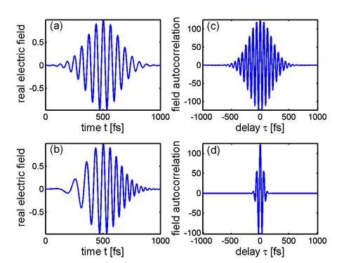Two ultrashort pulses (a) and (b) with their respective field autocorrelation (c) and (d). Note that the autocorrelations are symmetric and peak at zero delay. Note also that unlike pulse (a), pulse (b) exhibits an instantaneous frequency sweep, called chirp, and therefore contains more bandwidth than pulse (a). Therefore, the field autocorrelation (d) is shorter than (c), because the spectrum is the Fourier transform of the field autocorrelation (Wiener-Khinchin theorem).

Intensity autocorrelation

To a complex electric field E(t) corresponds an intensity I(t) = | E(t) | ² and an intensity autocorrelation function defined by

$A(\tau) = \int_{-\infty}^{+\infty}I(t)I(t-\tau)dt$

The optical implementation of the intensity autocorrelation is not as straightforward as for the field autocorrelation. Similarly to the previous setup, two parallel beams with a variable delay are generated, then focused into a second-harmonic-generation crystal (see nonlinear optics) to obtain a signal proportional to (E(t) + E(t − τ))². Only the beam propagating on the optical axis, proportional to the cross-product E(t)E(t − τ), is retained. This signal is then recorded by a slow detector, which measures

$I_M(\tau) = \int_{-\infty}^{+\infty}|E(t)E(t-\tau)|^2dt = \int_{-\infty}^{+\infty}I(t)I(t-\tau)dt$

I_M(τ) is exactly the intensity autocorrelation A(τ).

The generation of the second harmonic in crystals is a nonlinear process that requires high peak power, unlike the previous setup. However, such high peak power can be obtained from a limited amount of energy by ultrashort pulses, and as a result their intensity autocorrelation is often measured experimentally. Another difficulty with this setup is that both beams must be focused at the same point inside the crystal as the delay is scanned in order for the second harmonic to be generated.

It can be shown that the intensity autocorrelation width of a pulse is related to the intensity width. For a Gaussian time profile, the autocorrelation width is $\sqrt{2}$ longer than the width of the intensity, and it is 1.54 longer in the case of an hyperbolic secant squared (sech²) pulse. This numerical factor, which depends on the shape of the pulse, is sometimes called the deconvolution factor. If this factor is known, or assumed, the time duration (intensity width) of a pulse can be measured using an intensity autocorrelation. However, the phase cannot be measured.

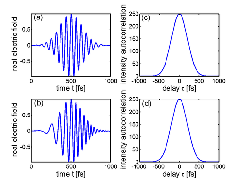Two ultrashort pulses (a) and (b) with their respective intensity autocorrelation (c) and (d). Because the intensity autocorrelation ignores the temporal phase of pulse (b) that is due to the instanteneous frequency sweep (chirp), both pulses yield the same intensity autocorrelation. Here, identical Gaussian temporal profiles have been used, resulting in an intensity autocorrelation width 2^1/2 longer than the original intensities. Note that an intensity autocorrelation has a background that is ideally half as big as the actual signal. The zero in this figure has been shifted to omit this background.

Interferometric autocorrelation

Setup for an interferometric autocorrelator, similar to the field autocorrelator above, with the following optics added: L: converging lens, SHG: second-harmonic generation crystal, F: spectral filter to block the fundamental wavelength.

As a combination of both previous cases, a nonlinear crystal can be used to generate the second harmonic at the output of a Michelson interferometer, in a colinear geometry. In this case, the signal recorded by a slow detector is

$I_M(\tau) = \int_{-\infty}^{+\infty}|(E(t)+E(t-\tau))^2|^2dt$

I_M(τ) is called the interferometric autocorrelation. It contains some information about the phase of the pulse: the fringes in the autocorrelation trace wash out as the spectral phase becomes more complex.

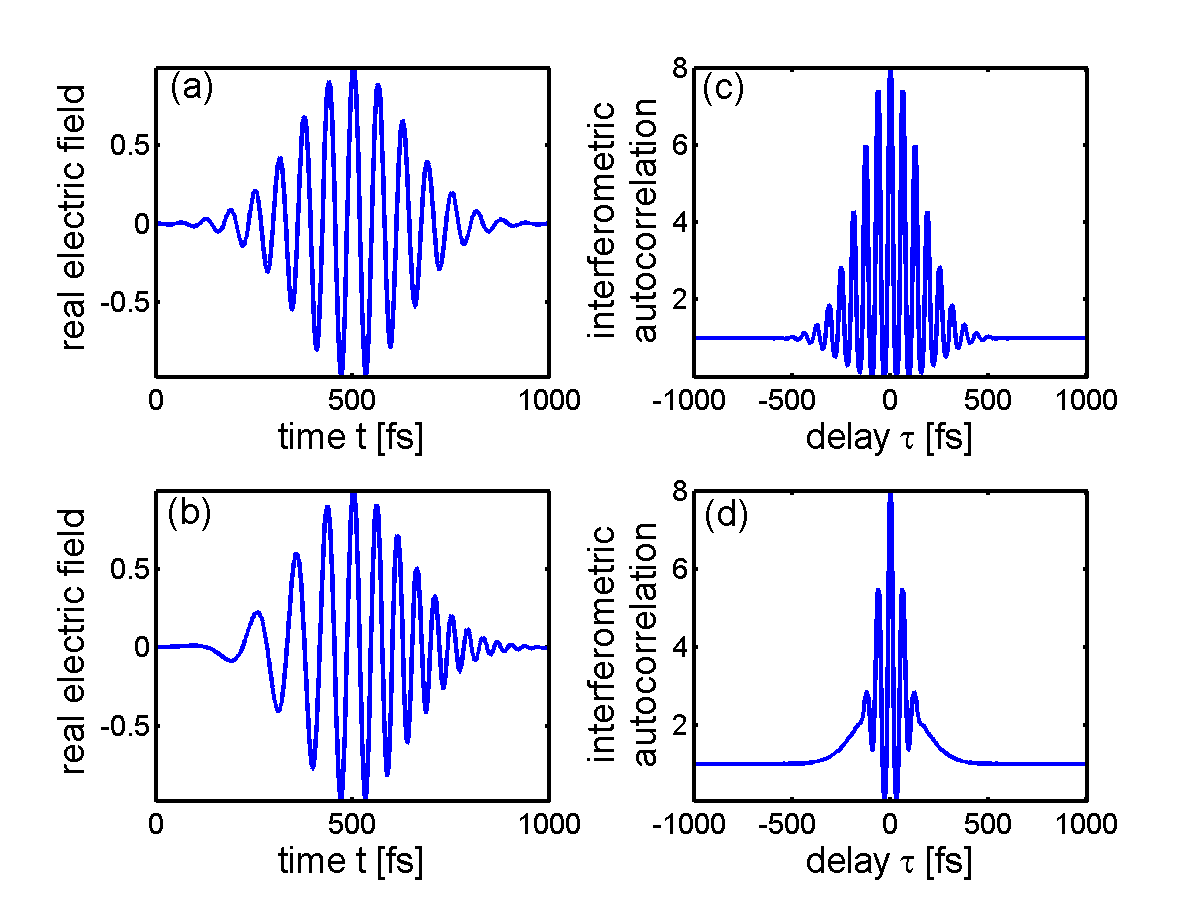
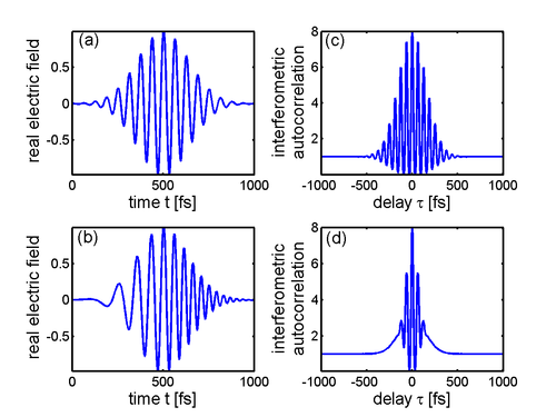Two ultrashort pulses (a) and (b) with their respective interferometric autocorrelation (c) and (d). Because of the phase present in pulse (b) due to an instantaneous frequency sweep (chirp), the fringes of the autocorrelation trace (d) wash out in the wings. Note the ratio 8:1 (peak to the wings), characteristic of interferometric autocorrelation traces.

Pupil function autocorrelation

The optical transfer function T(w) of an optical system is given by the autocorrelation of its pupil function f(x,y):

$T(w) = \frac{\int_{w/2}^{1} \int_{0}^{\sqrt{1-x^2}} f(x,y) f^*(x-w,y)dy dx}{\int_{0}^{1}\int_{0}^{\sqrt{1-x^2}}f(x,y)^2 dy dx}$

See also

• Autocorrelator
• Convolution

References

1. ^ Roth, J. M., Murphy, T. E. & Xu, C. Ultrasensitive and high-dynamic-range two-photon absorption in a GaAs photomultiplier tube, Opt. Lett. 27, 2076–2078 (2002).
2. ^ J. C. Diels and W. Rudolph, Ultrashort Laser Pulse Phenomena, 2nd Ed. (Academic, 2006).
3. ^ W. Demtröder, Laserspektroscopie: Grundlagen und Techniken, 5th Ed. (Springer, 2007).