Chaotic mixing

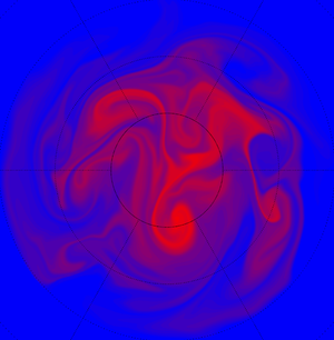An example of chaotic mixing

In chaos theory and fluid dynamics, chaotic mixing is a process by which flow tracers develop into complex fractals under the action of a time-varying fluid flow. The flow is characterized by an exponential growth of fluid filaments. ^[1] Even very simple flows, such as the blinking vortex, or finitely resolved wind fields can generate exceptionally complex patterns from initially simple tracer fields. ^[2]

The phenomenon is still not well understood and is the subject of much current research.

Measuring filament growth

Lyapunov exponents

A trajectory in the fluid is determined by the following system of ordinary differential equations:

$\frac{d \vec x}{dt} = \vec v(\vec x, t)$

where $\vec x$ is the physical position, t is time, and $\vec v$ is the fluid velocity as a function of both position and time. If the flow is chaotic, then small initial errors in a trajectory will diverge exponentially. We are interested in calculating the stability—i.e., how fast do nearby trajectories diverge? Suppose we make a small perturbation, $\delta \vec{x}$, then using a Taylor expansion, we get:

$\frac {\mathrm d} {\mathrm dt} (\vec{x}+\delta \vec{x}) \approx \vec{v} + \nabla \vec{v} \cdot \delta \vec{x}$

The Jacobi matrix of the velocity field, $\nabla \vec{v}$, provides information about the local rate of divergence of nearby trajectories or the local rate of stretching of Lagrangian space. The rate of change of the error vectors is given approximately as:

$\frac {\mathrm d} {\mathrm dt} \delta \vec x \approx \nabla \vec v \cdot \delta \vec x$

We define the matrix H such that:

$\frac {\mathrm d} {\mathrm dt} \boldsymbol{H} \equiv \nabla \vec{v} \cdot \boldsymbol{H}, \qquad \boldsymbol{H} (t=0)=\boldsymbol{I}$

where I is the identity matrix. It follows that:

$\delta \vec{x} (t) \approx \boldsymbol{H} \cdot \delta \vec{x}_0$

The Lyapunov exponents are defined as the time average of the logarithms of the lengths of the principal components of the vector H in the limit as t approaches infinity:

$\boldsymbol{H^T} \cdot \boldsymbol{H} \cdot \delta \vec{x}_{0i} = h_i \cdot \delta \vec{x}_{0i}$

$\lambda_i \equiv \lim_{t \to \infty} \frac {1} {2 t} \ln {h_i}$

where $\lambda_i \geq \lambda_{i+1}$ is the ith Lyapunov exponent of the system, while $\delta \vec {x}_{0i}$ is the ith principal component of the matrix H.

If we start with a set of orthonormal initial error vectors, $\{\delta \vec x_{0i}\}$ then the matrix H will map them to a set of final orthogonal error vectors of length $\{\sqrt{h_i}\}$. The action of the system maps an infinitesimal sphere of inititial points to an ellipsoid whose major axis is given by the $\sqrt{h_1}$ while the minor axis is given by $\sqrt{h_N}$, where N is the number of dimensions. ^{[3] [4]}

This definition of Lyapunov exponents is both more elegant and more appropriate to real-world, continuous-time dynamical systems than the more usual definition based on discrete function maps. Chaos is defined as at least one positive Lyapunov exponent.

If there is any significant difference between the Lyapunov exponents then as an error vector evolves forward in time, any displacement in the direction of largest growth will tend to be magnified. Thus:

$|\delta \vec x| \approx |\delta \vec x_0| e^{\lambda_1 t}$

where λ₁ is the largest Lyapunov exponent. In fact, the Lyapunov exponent is often somewhat incorrectly defined in this way. ^[4]

Contour advection

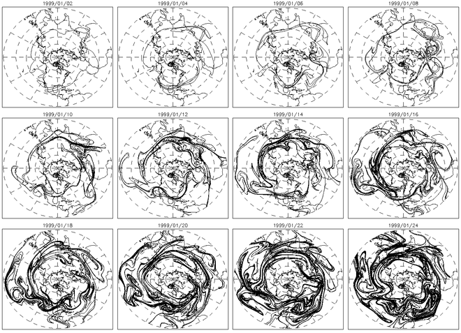Evolution of an advected contour

Contour advection is another useful method for characterizing chaotic mixing. In chaotic flows, advected contours will grow exponentially over time. The figure above shows the frame-by-frame evolution of a contour advected over several days. The figure to the right shows the length of this contour as a function of time.

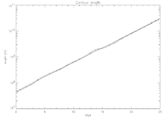Growth of advected contour

The link between exponential contour growth and positive Lyapunov exponents is easy to see. The rate of contour growth is given as:

$\frac{\mathrm d L}{\mathrm d t} = \int | \nabla \vec v \cdot \mathrm d \vec s |$

where $\mathrm d \vec s$ is the path and the integral is performed over the length of the contour. Contour growth rates will approximate the average of the large Lyapunov exponents: ^[3]

$L \approx L_0 \exp(\bar \lambda_1 t)$

Fractal dimension

Through a continual process of stretching and folding, much like in a "baker's map," tracers advected in chaotic flows will develop into complex fractals. The fractal dimension of a single contour will be between 1 and 2. Exponential growth ensures that the contour, in the limit of very long time integration, becomes fractal. Fractals composed of a single curve are infinitely long and when formed iteratively, have an exponential growth rate, just like an advected contour. The Koch Snowflake, for instance, grows at a rate of 4/3 per iteration.

The figure below shows the fractal dimension of an advected contour as a function of time, measured in four different ways. A good method of measuring the fractal dimension of an advected contour is the uncertainty exponent.

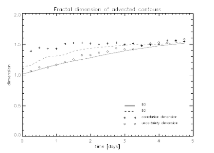Advected contour fractal dimension^[3]

External links

• ctraj: Tools for studying chaotic advection.

References

1. ^ J. M. Ottino (1989). The Kinematics of Mixing: Stretching, Chaos and Transport. Cambridge University Press. 
2. ^ J. Methven and B. Hoskins (1999). "The advection of high-resolution tracers by low-resolution winds". Journal of the Atmospheric Sciences 56 (18): 3262–3285. 
3. ^ ^{a b c} Peter Mills (2004). Following the Vapour Trail: a Study of Chaotic Mixing of Water Vapour in the Upper Troposphere (Thesis). http://www.sat.ltu.se/members/pmils/Masters_Thesis_Peter_reduced.pdf. 
4. ^ ^{a b} Edward Ott (1993). Chaos in Dynamical Systems. Cambridge University Press.